Lesson 2

library(dplyr)
library(magrittr)
library(ggplot2)
library(tidyr)
theme_set(theme_minimal())

Some technical Stan stuff

• Back to Task 4 from past lesson
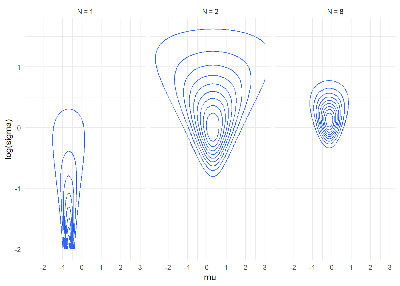
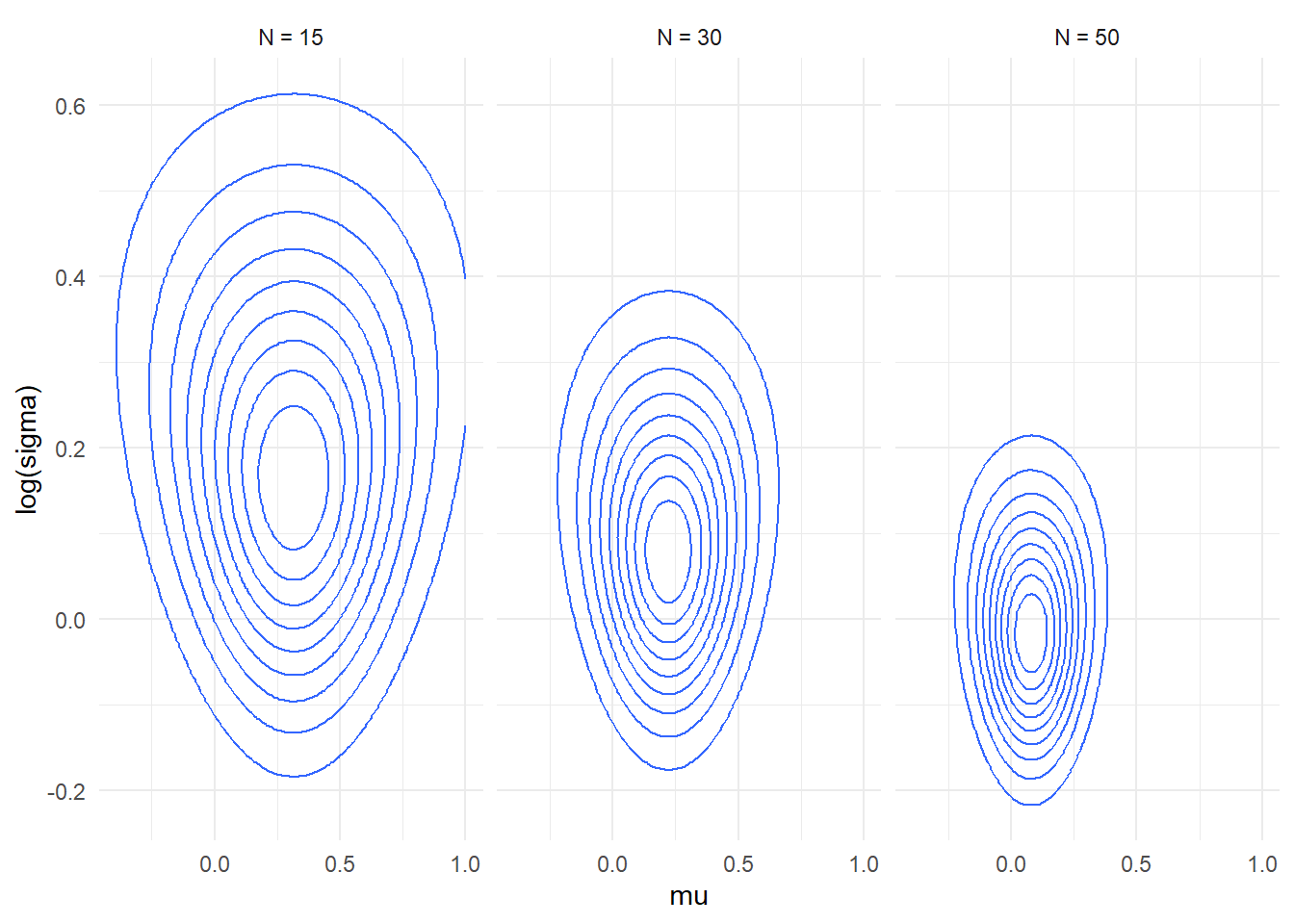
  • Here is a plot of how likelihood of the simple normal model with unknown mean and standard deviation changes as we add data points. Note that for N=1 the plot is truncated as the density grows without bounds as \(\log \sigma \to \infty\) and \(\mu \to y_1\).
  • The plots don’t include prior, just the likelihood. Prior improves things a bit, but not enough (as witnessed by the warnings from Stan)
  • Note that the likelihood is still visibly skewed (and thus non-normal) even for quite large datasets.

plot_densities <- function(n_data_vals, mu_range = c(-3,3), log_sigma_range = c(-2,2)) {
  set.seed(566522)
  y = c(-0.6906332,  1.2873201, 2.0089285, 0.1347772, -0.8905993, -0.8171846, rnorm(max(1, max(n_data_vals))))
  underdetermined_theory <- crossing(mu = seq(mu_range[1], mu_range[2], length.out = 200), log_sigma = seq(log_sigma_range[1], log_sigma_range[2], length.out = 200),
           data.frame(y_id = 1:length(y), y = y), n_data = n_data_vals
           ) %>%
    filter(y_id <= n_data) %>%
    mutate(log_density_point = dnorm(y, mu, exp(log_sigma), log = TRUE)) %>%
    group_by(mu, log_sigma, n_data) %>%
    summarise(log_density = sum(log_density_point), .groups = "drop") %>%
    group_by(n_data) %>%
    mutate(rel_density = exp(log_density - max(log_density))) %>%
    ggplot(aes(x = mu, y = log_sigma, z = rel_density)) + geom_contour() + #geom_raster() + 
    facet_wrap(~n_data, nrow = 1, labeller = label_bquote(cols = paste(N, " = ", .(n_data)) )) + scale_y_continuous("log(sigma)")
  
  underdetermined_theory
}

plot_densities(c(1,2,8))

plot_densities(c(15, 30, 50), mu_range = c(-1,1), log_sigma_range = c(-0.5,1))

• Explain divergences - we will mostly follow https://mc-stan.org/misc/warnings
  • Divergences are your friend!
• Sampling statements vs. target increments (https://mc-stan.org/docs/reference-manual/statements.html#sampling-statements.section)
  • “Up to a constant” - recall the half-normal prior for sigma.
  • xx_lupdf, xx_lupmf

Using integers in Stan programs

• Ints can only ever be data
• Arrays are declared as array[size] base_type; (arrays in Stan manual)
  • i.e. array of N ints is array[N] int;
  • You can have arrays of anything (i.e. vectors, matrices, bounded integers, …)
• Poisson and negative binomial distibution
  • Modelling log mean
  • The mean - overdispersion parametrization of negative binomial
    • In R, you can use rnbinom(mu = mean, size = overdispersion)
    • In Python, it seems you need to convert manually, see https://stackoverflow.com/a/62460072/802009 for Python

Workflow

• We will follow the Bayesian workflow from https://arxiv.org/abs/2011.01808 - we’ll start with the most useful and simple steps in this lesson.
• Build slowly and test as many assumptions of the model as possible
  • The assumptions will usually be wrong. But are they importantly wrong?
• The goal is to be able to confidently build complex models
• Steps of modelling, that need to be checked:
  • Prior, fit to data (likelihood), computation
  • Checking parameter recovery from simulations is a simple computation check
• Priors can (and should) be tested: prior predictive check
  • Simulate data from the prior, check that the data match domain expertise
  • If they don’t the prior is bad
    • It may however be unclear how to get a better prior…
• Posterior predictive checks:
  • Compute something about a dataset (e.g. variance for each group of observations)
  • Copmute the same something about each posterior draw
  • If the values for the actual dataset lie in the extreme of the posterior distribution, something is wrong
• Simple model first. Individual components first separately, then joined.