Simple Bernoulli Examples

Abstract

This R Markdown document runs the simulations accompanying Examples 1 - 5 in Appendix B of paper ‘Simulation-Based Calibration Checking for Bayesian Computation: The Choice of Test Quantities Shapes Sensitivity’

The examples are run using the SBC R package. - consult the Getting Started with SBC vignette for basics of the package. We will also use “custom backends” which are discussed and explaiend in the Implementing a new backend.

knitr::opts_chunk$set(cache = TRUE)
library(SBC)
library(tidyverse)
library(patchwork)

library(future)
plan(multisession)

theme_set(cowplot::theme_cowplot())

# Setup cache
cache_dir <- "./_SBC_cache_bernoulli"
if(!dir.exists(cache_dir)) {
  dir.create(cache_dir)
}

Recall that the model is:

\[ \begin{align} \Theta &:= \mathbb{R} \notag\\ Y &:= \{0,1\} \notag\\ \theta &\sim \mathrm{uniform}(0,1) \notag\\ y &\sim \mathrm{Bernoulli}(\theta) .\label{eq:bernoulli_model} \end{align} \]

First, we generate a large number of datasets:

set.seed(1558655)

N_sims_simple <- 1000
N_sims_simple_large <- 10000
N_samples_simple <- 100

variables_simple <- runif(N_sims_simple_large)
generated_simple <- 
  purrr::map(variables_simple, ~ list(y = rbinom(1, size = 1, .x)))

ds_large <- SBC_datasets(variables = posterior::draws_matrix(theta = variables_simple),
                               generated = generated_simple)

ds <- ds_large[1 : N_sims_simple]

We then create two simple classes of SBC backends. First (my_backend_func) just uses one function to generate samples when \(y = 0\) and another when \(y = 1\). The second one (my_backend_func_invcdf) is very similar, but takes the inverse CDF functions for \(y = 0\) and \(y = 1\) as input.

my_backend_func <- function(func0, func1) {
  structure(list(func0 = func0, func1 = func1), class = "my_backend_func")
}

SBC_fit.my_backend_func <- function(backend, generated, cores) {
  if(generated$y == 0) {
    posterior::draws_matrix(theta = backend$func0())
  } else if (generated$y == 1) {
    posterior::draws_matrix(theta = backend$func1())
  } else {
    stop("Invalid")
  }
}

SBC_backend_iid_draws.my_backend_func <- function(backend) {
  TRUE
}

my_backend_func_invcdf <- function(invcdf0, invcdf1) {
  structure(list(invcdf0 = invcdf0, invcdf1 = invcdf1), class = "my_backend_func_invcdf")
}

SBC_fit.my_backend_func_invcdf <- function(backend, generated, cores) {
  if(generated$y == 0) {
    posterior::draws_matrix(theta = backend$invcdf0(runif(N_samples_simple)))
  } else if (generated$y == 1) {
    posterior::draws_matrix(theta = backend$invcdf1(runif(N_samples_simple)))
  } else {
    stop("Invalid")
  }
}

SBC_backend_iid_draws.my_backend_func_invcdf <- function(backend) {
  TRUE
}


my_globals <- c("SBC_fit.my_backend_func", "SBC_backend_iid_draws.my_backend_func", "SBC_fit.my_backend_func_invcdf",
                "SBC_backend_iid_draws.my_backend_func_invcdf", "N_samples_simple")

Finally, we set a range of test quantities to monitor:

gq_simple <- derived_quantities(
   log_lik = dbinom(y, size = 1, prob = theta, log = TRUE),
   sq = (theta - 0.5) ^ 2,
   sin3_2 = sin(3/2 * pi * theta),
   saw = ifelse(theta < 1/2, theta, -1/2 + theta),
   swap = ifelse(theta < 1/2, theta, theta - 1),
   saw_quad = ifelse(theta < 1/2, theta^2, -1/2 + theta^3),
   clamp = ifelse(theta < 1/2, theta, 1/2)
   # CRPS was suggested, but seems not really useful
   # Following equation (8) at https://arxiv.org/pdf/2002.09578v1.pdf for CRPS
   # CRPS = (1 - dbinom(y, size = 1, prob = theta)) - 0.5 * dbinom(1, size = 2, prob = theta)
   )

Correct posterior

Setup a backend using the correct analytic posterior - it passes SBC including all GQs

backend_ok <- my_backend_func(
  func0 = rlang::as_function(~ rbeta(N_samples_simple, 1, 2)),
  func1 = rlang::as_function(~ rbeta(N_samples_simple, 2, 1)))


res_ok <- compute_SBC(ds, backend_ok, keep_fits = FALSE,
                      dquants = gq_simple, globals = my_globals,
                      cache_mode = "results",
                      cache_location = file.path(cache_dir, "ok")
)

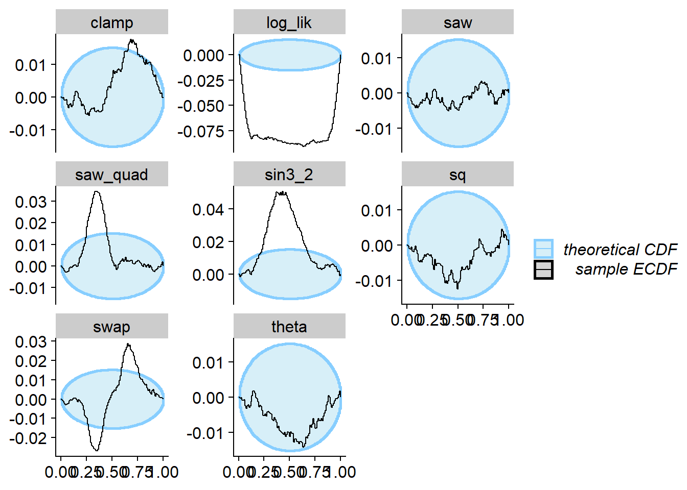
## Results loaded from cache file 'ok'

plot_rank_hist(res_ok)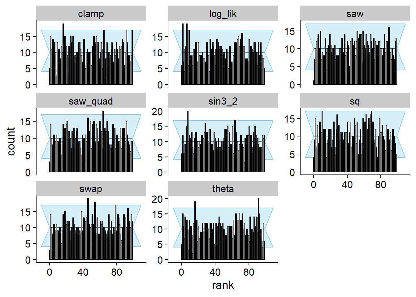

plot_ecdf_diff(res_ok)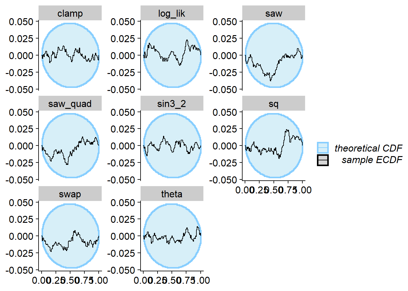

Example 1 - Projection

We now demonstrate some incorrect posteriors that however satisfy SBC w.r.t. the projection function (\(f_1\) in the paper, theta in the code and plots here). The counterexamples are most naturally expressed vie inverse CDFs, so for this and all the following examples, we will show the inverse CDFs. For the first counterexample we will take \(\Phi^{-1}(x | 0) = x^2\) and then use the formula \(\Phi^{-1}(x | 1) = \sqrt{2x + (\Phi^{-1}(x | 0) - 1)^2 - 1}\) to calculate the other inverse CDF.

invcdf_ex1_square_0 <- function(u) {
  u^2
}

invcdf_ex1_square_1 <- function(u) {
  sqrt(u * (2-2*u+u^3))
}

This is how the inverse CDFs of the counterexample compare to the correct ones - the top two panels show the actual inverse CDFs and the bottom two panels the difference from the correct CDF.

plot_invcdfs <- function(invcdf0, invcdf1, name) {
  u <- seq(from = 0, to = 1,length.out = 100)
  plot1 <- rbind(data.frame(y = 0, u = u, invphi = invcdf0(u), type = name),
        data.frame(y = 1, u = u, invphi = invcdf1(u), type = name),
        data.frame(y = 0, u = u, invphi = 1 - sqrt(1 - u), type = "Correct"),
        data.frame(y = 1, u = u, invphi = sqrt(u), type = "Correct")
        ) %>%
    ggplot(aes(x = u, y = invphi, color = type)) + geom_line(size = 2) + facet_wrap(~y, labeller = label_both) +
    scale_y_continuous("Inverse CDF of theta") +
    scale_x_continuous("Quantile")
  
  plot2 <- 
    rbind(data.frame(y = 0, u = u, invphi_diff = invcdf0(u) - ( 1 - sqrt(1 - u)), type = name),
        data.frame(y = 1, u = u, invphi_diff = invcdf1(u) - sqrt(u), type = name),
        crossing(y = c(0,1), u = u, invphi_diff = 0, type = "Correct")) %>%
    ggplot(aes(x = u, y = invphi_diff, color = type)) + geom_line(size = 2) + facet_wrap(~y, labeller = label_both) +
    scale_y_continuous("Diff. inverse CDF of theta") +
    scale_x_continuous("Quantile")
  
  plot1 / plot2
}

plot_invcdfs(invcdf_ex1_square_0, invcdf_ex1_square_1, "Example 1 - Square")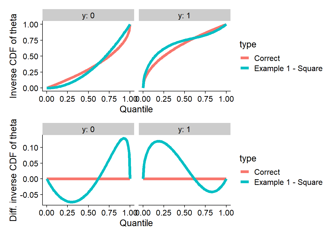

Now we can run SBC. We see that for theta SBC passes with no problems while for all the other test quantities it fails.

backend_ex1_square <- my_backend_func_invcdf(invcdf_ex1_square_0, invcdf_ex1_square_1)


res_ex1_square <- compute_SBC(ds_large, backend_ex1_square, keep_fits = FALSE,
                        dquants = gq_simple, globals = my_globals,
                      cache_mode = "results",
                      cache_location = file.path(cache_dir, "ex1_square"))

## Cache file exists but the backend hash differs. Will recompute.

plot_rank_hist(res_ex1_square)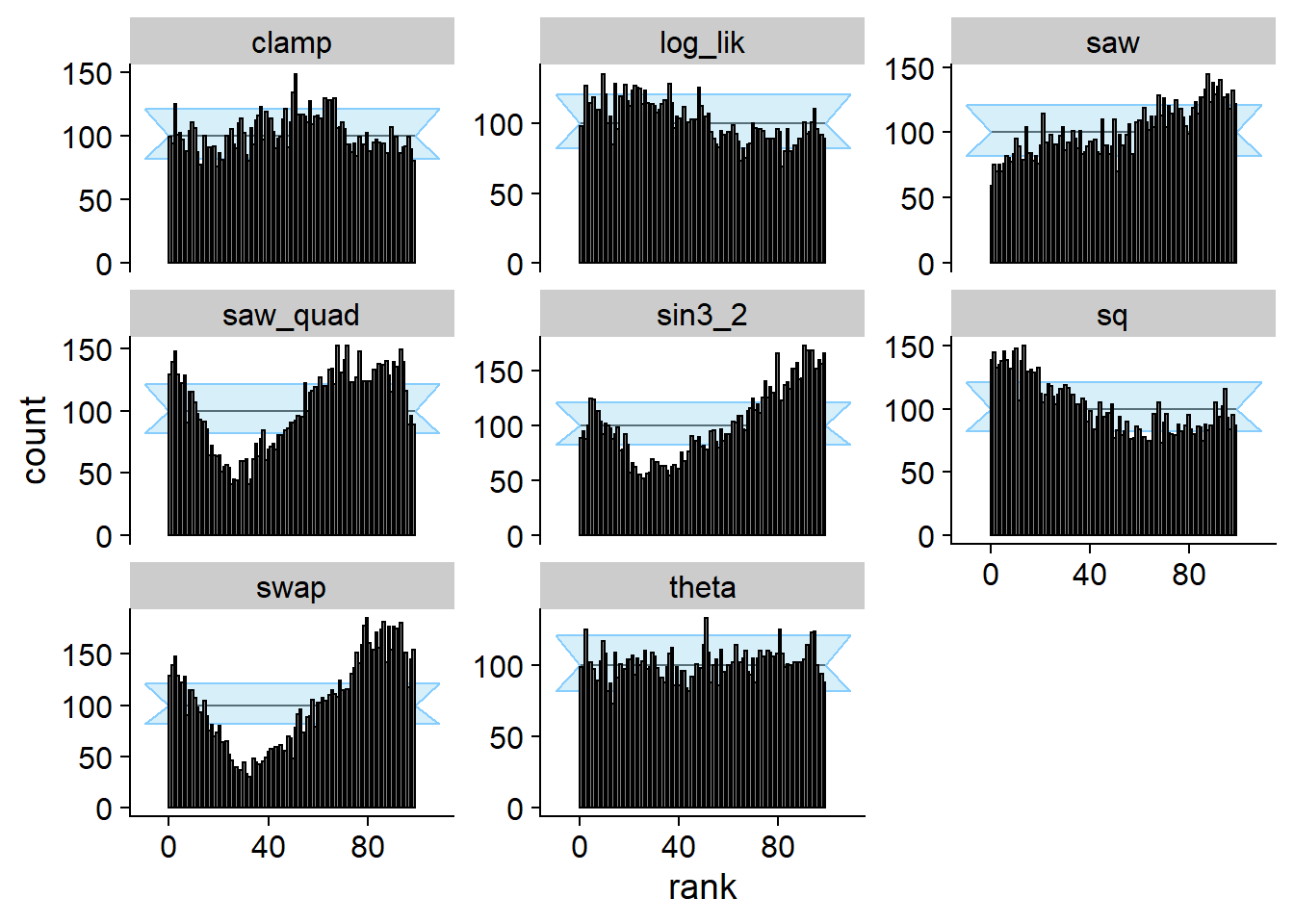

plot_ecdf_diff(res_ex1_square)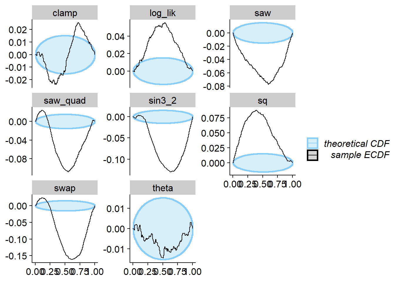

Example 2 - Projection and Data-Averaged Posterior

Flipped 0 and 1 outcomes

Here we take the correct posterior and flip the functions for 0 and 1. In paper, this is designated as \(\phi_A\). This still satisfies the “data-averaged posterior = prior” condition but actually fails SBC for the projection function (i.e. the theta subplot) and many other test quantities. Interestingly, the sq quantity is completely insensitive to this flipping, because it is symmetric to flips in theta around \(\frac{1}{2}\).

backend_flip <- my_backend_func(
  func0 = rlang::as_function(~ rbeta(N_samples_simple, 2, 1)),
  func1 = rlang::as_function(~ rbeta(N_samples_simple, 1, 2)))


res_flip <- compute_SBC(ds, backend_flip, keep_fits = FALSE,
                        dquants = gq_simple, globals = my_globals)

plot_rank_hist(res_flip)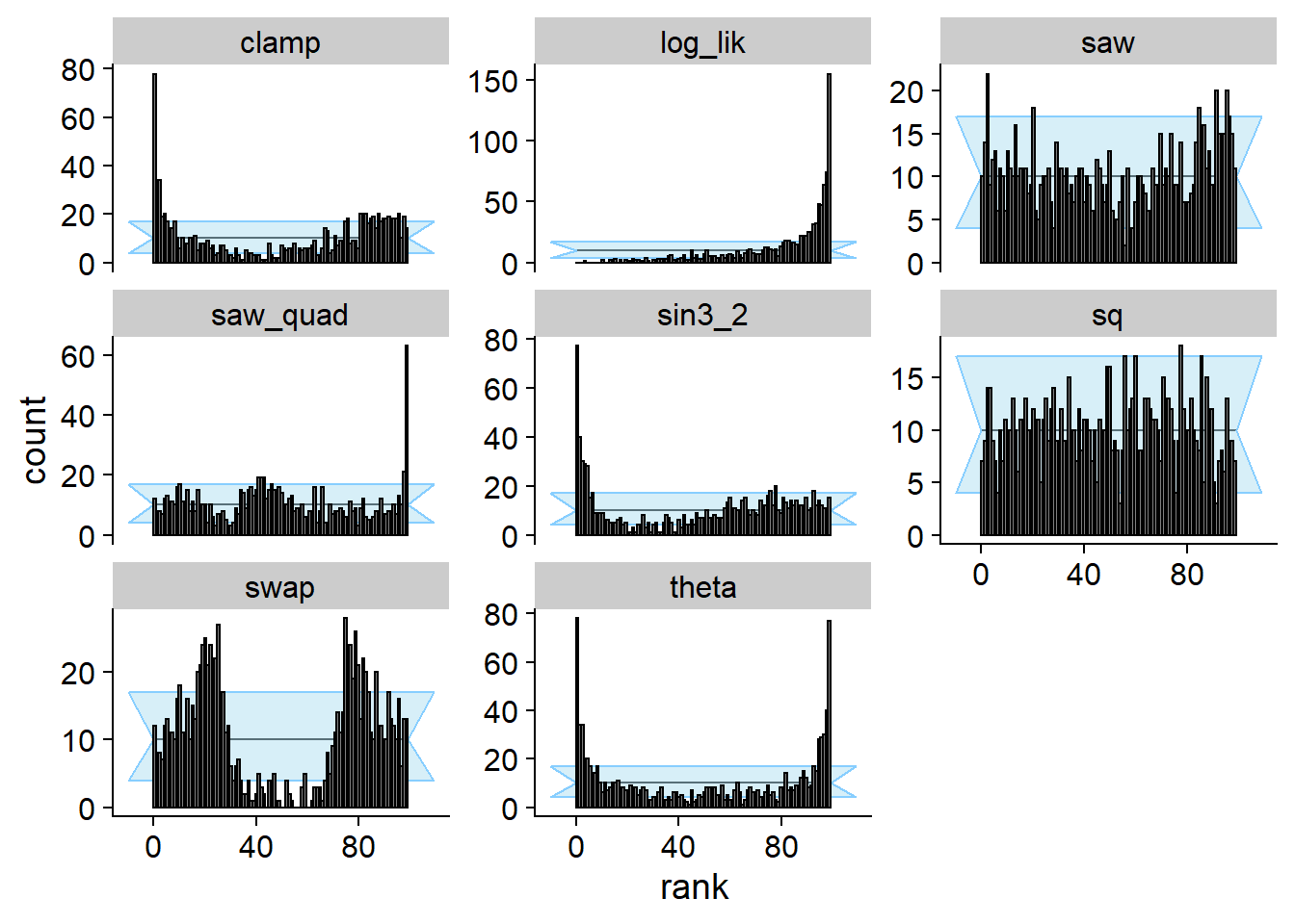

plot_ecdf_diff(res_flip)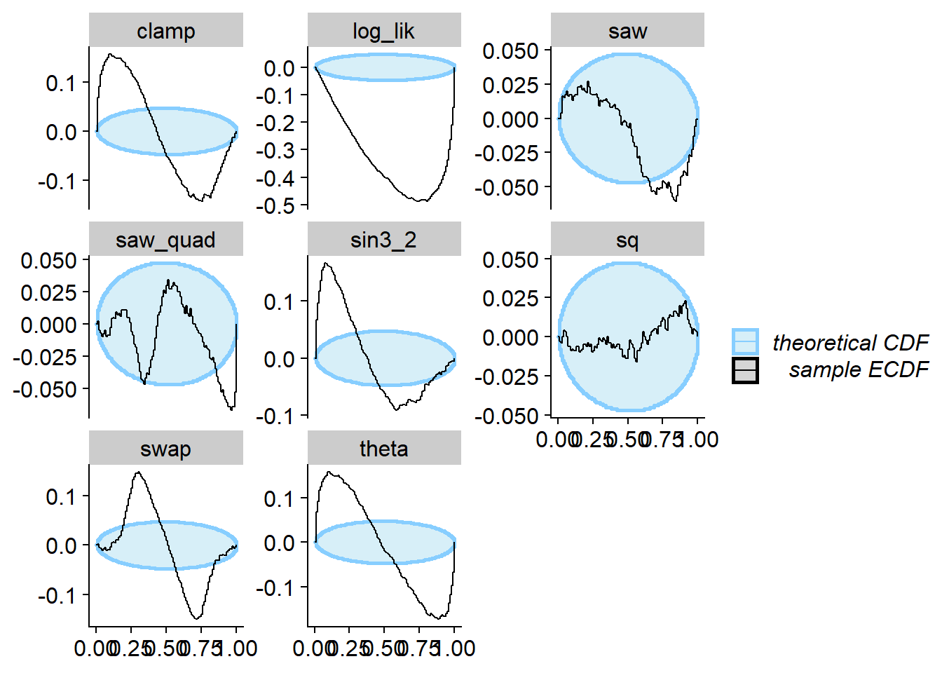

Satisfy SBC, fail data-averaged posterior

Now, we recreate the example denoted \(\Phi_B\) in the paper - we take

\[ \Phi^{-1}_B(x | 0) := \begin{cases} \frac{2}{3}x & x < \frac{3}{4} \\ \frac{1}{2} + 2(x - \frac{3}{4}) & x \geq \frac{3}{4} \\ \end{cases} \\ \]

and then use the formula \(\Phi^{-1}(x | 1) = \sqrt{2x + (\Phi^{-1}(x | 0) - 1)^2 - 1}\) to calculate the other inverse CDF.

invcdf_phiB_0 <- function(u) {
  ifelse(u < 3/4, (2/3) * u, 0.5 + (u - 0.75)*2)
}

invcdf_phiB_1 <- function(u) {
  ifelse(u < 3/4, (1/3) * sqrt(2) * sqrt(u * (3 + 2 * u)), sqrt(3 - 6*u + 4*u^2))
}


plot_invcdfs(invcdf_phiB_0, invcdf_phiB_1, "Example 2 - phiB")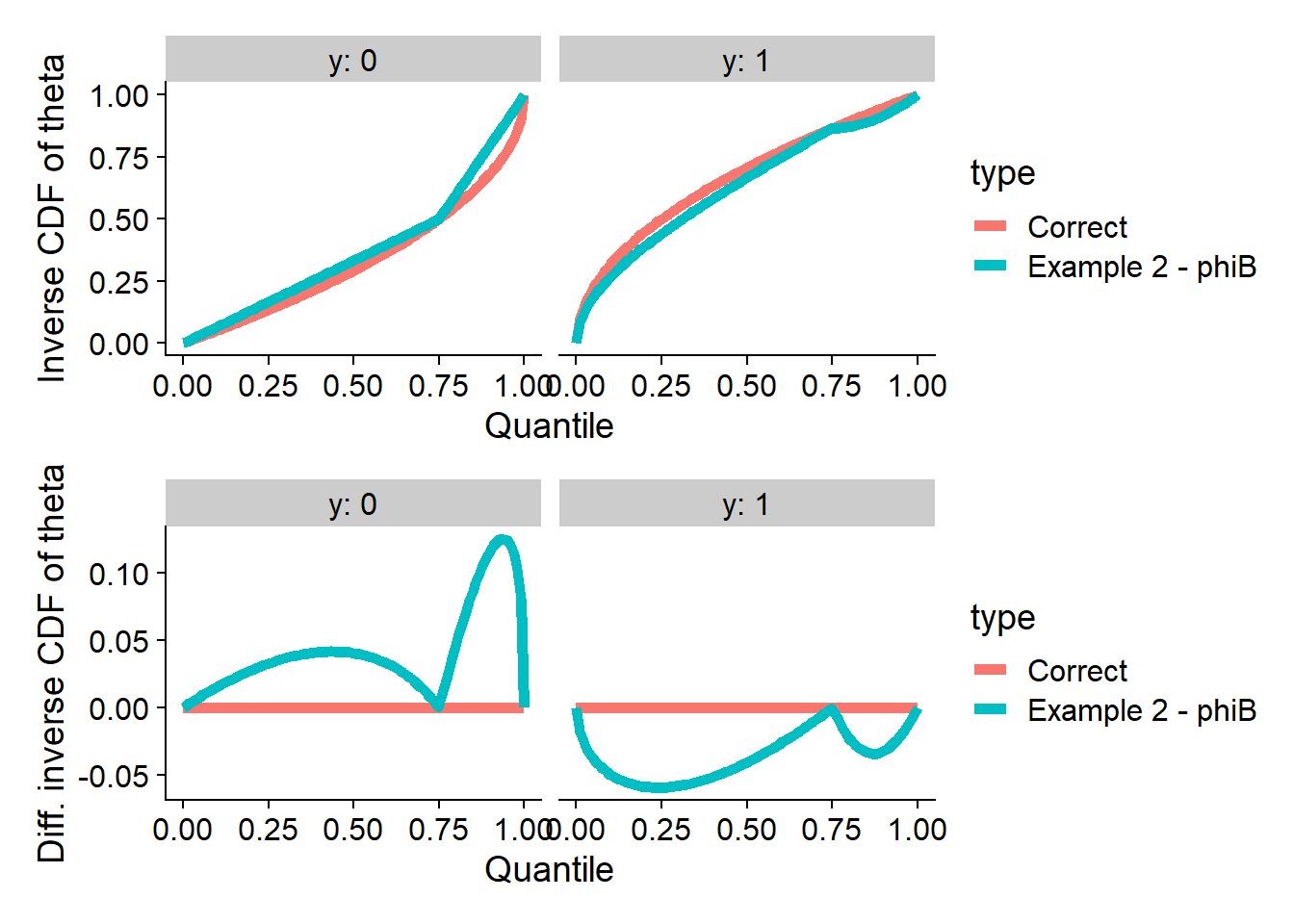

Let’s run SBC. As designed, no problem with theta (projection function), but many test quantities signal problems.

backend_phiB <- my_backend_func_invcdf(invcdf_phiB_0, invcdf_phiB_1)


# We use a bit more simulations to clearly show some of the problems
res_phiB <- compute_SBC(ds_large[1:2500], backend_phiB, keep_fits = FALSE,
                        dquants = gq_simple, globals = my_globals,
                      cache_mode = "results",
                      cache_location = file.path(cache_dir, "phiB")
                        )

## Cache file exists but the backend hash differs. Will recompute.

plot_rank_hist(res_phiB)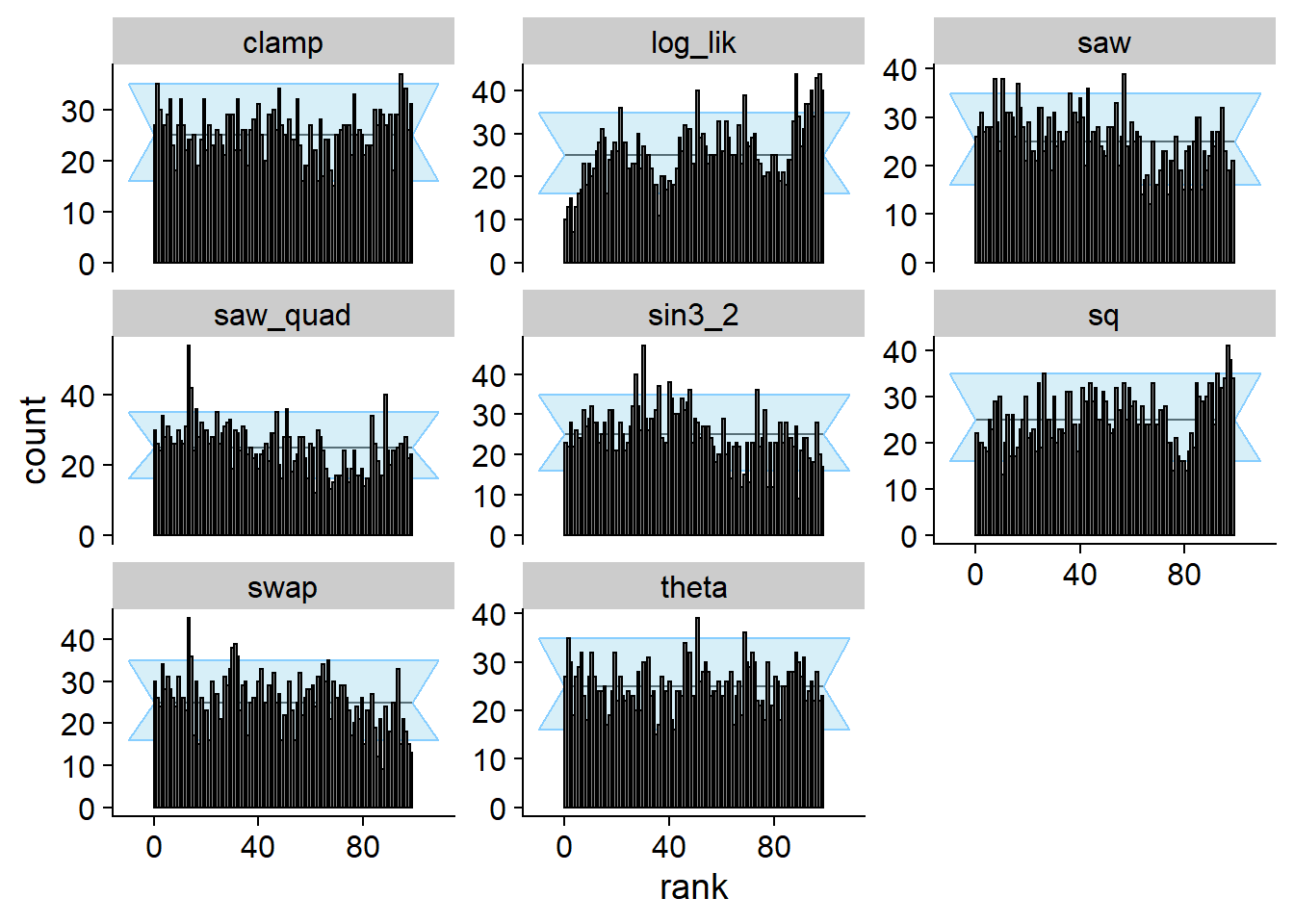

plot_ecdf_diff(res_phiB)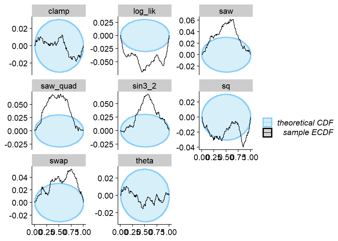

Linear combinations

Here we take a linear combination of the prior and posterior (both passing SBC and data-averaged posterior for theta - the projection function). This is denoted as \(\Phi_C\) in the paper. Note that this does not quite strongly pass SBC for theta (the projection function) as well as many other quantities.

invcdf_lincomb_0 <- function(u) {
  1.5 - 0.5 * sqrt(9 - 8 * u)
}

invcdf_lincomb_1 <- function(u) {
  -0.5 + 0.5 * sqrt(1 + 8 * u)
}

plot_invcdfs(invcdf_lincomb_0, invcdf_lincomb_1, "Linear combination")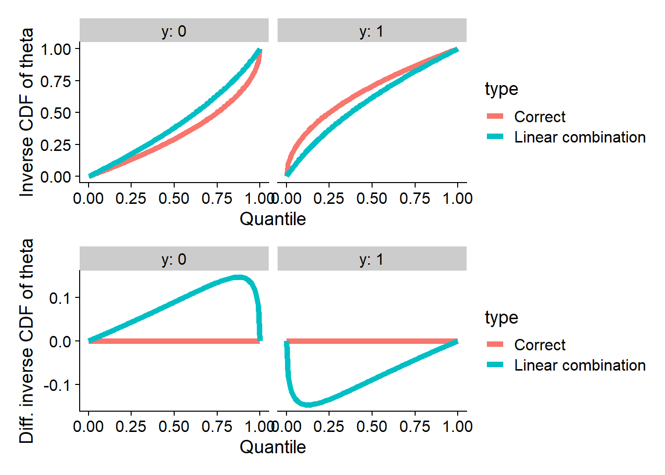

backend_lincomb <- my_backend_func_invcdf(invcdf_lincomb_0, invcdf_lincomb_1)


res_lincomb <- compute_SBC(ds_large, backend_lincomb, keep_fits = FALSE,
                        dquants = gq_simple, 
                        globals = my_globals,
                      cache_mode = "results",
                      cache_location = file.path(cache_dir, "lincomb"))

## Cache file exists but the backend hash differs. Will recompute.

plot_rank_hist(res_lincomb)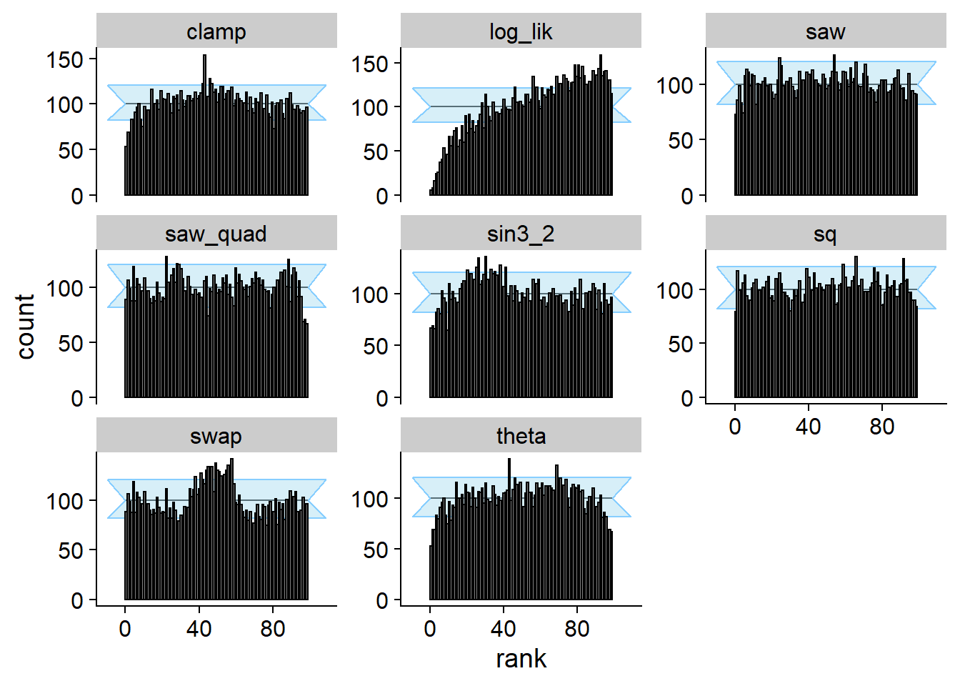

plot_ecdf_diff(res_lincomb)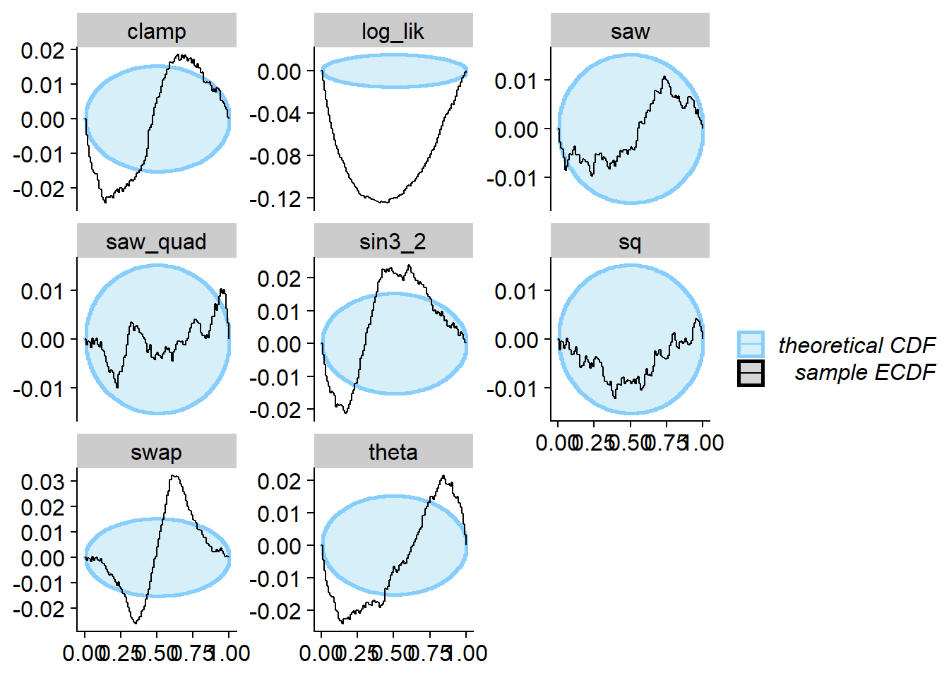

Example 3 - Likelihood

Now let us simulate posteriors passing SBC w.r.t. the likelihood (denoted \(f_2\) in the paper).

Passing SBC just for likelihood

Here we will use \(\Phi^{-1}(x | 1) = 1 - (1 - x)^2\) and then use the formula \(\Phi^{-1}(1 - x | 0) = 1 - \sqrt{2x - (\Phi^{-1}(x|1) ^ 2)}\) to complete the posterior.

invcdf_lik1_0 <- function(u) {
  #1 - sqrt((1 - u))
  #1 - sqrt(2*(1-u) - invcdf_lik1_1(1-u) ^ 2)
  1 - sqrt(1-u*(2 - 2*u + u^3))
}

invcdf_lik1_1 <- function(u) {
   1 - (1 - u)^2
}

plot_invcdfs(invcdf_lik1_0, invcdf_lik1_1, "Example 3 - Likelihood 1")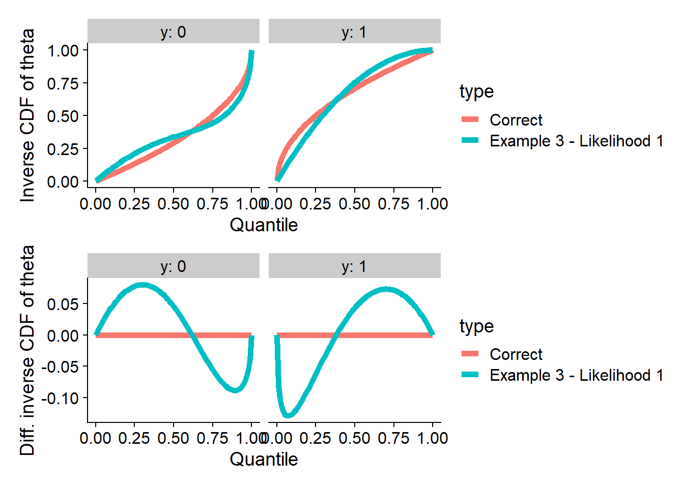

And we can compute SBC - note that this posterior passes SBC for the likelihood (log_lik), but it does not pass it for theta and many other quantities.

backend_lik1 <- my_backend_func_invcdf(invcdf_lik1_0, invcdf_lik1_1)

res_lik1 <- compute_SBC(ds, backend_lik1, keep_fits = FALSE,
                        dquants = gq_simple, globals = my_globals,
                      cache_mode = "results",
                      cache_location = file.path(cache_dir, "loglik1"))

## Cache file exists but the backend hash differs. Will recompute.

plot_rank_hist(res_lik1)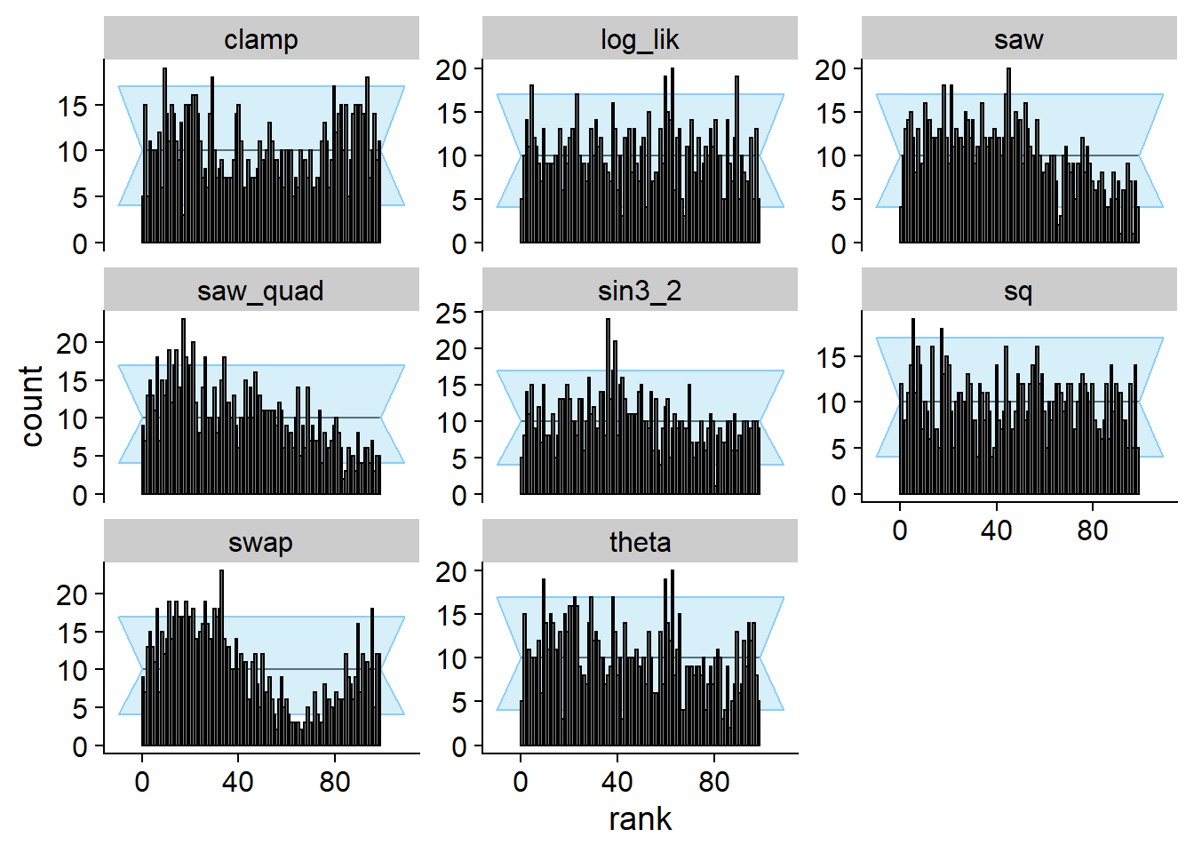

plot_ecdf_diff(res_lik1)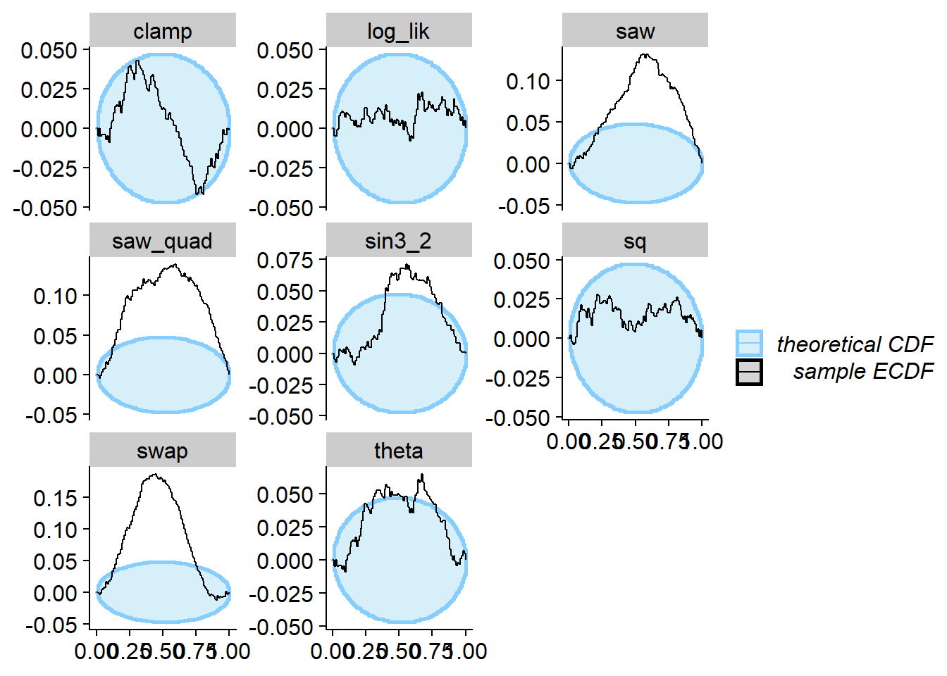

Passing SBC for both projection and likelihood

We can construct counterexamples that satisfy both theta and log_lik, the full formula is in the paper here is one, starting from \(0 < x < \frac{1}{2}: \Phi^{-1}(x | 0) = 2 (2 - \sqrt{2}) u^2\) and computing the rest as needed:

invcdf_loglik2_0 <- function(u) {
  ifelse(u < 0.5, u^2 * 2 *(2 - sqrt(2)),
           1 - 2 * abs(u - 1) * sqrt(-4 + 3 * sqrt(2) + (-6 + 4*sqrt(2)) * (u -2) * u) 
           )  
} 

invcdf_loglik2_1 <- function(u) {
  ifelse(u < 0.5, sqrt(2 * u *(1 + 2*u *(-2 + sqrt(2) + (6 - 4*sqrt(2)) * u^2))),
           sqrt(-17 + 12 * sqrt(2) + 2 * u * (41 - 28 * sqrt(2) + 2 * u * (-34 + 23 * sqrt(2) + (-6+4*sqrt(2)) * (u - 4) * u))))
}

plot_invcdfs(invcdf_loglik2_0, invcdf_loglik2_1, "Example 3 - likelihood 2")

## Warning in sqrt(-17 + 12 * sqrt(2) + 2 * u * (41 - 28 * sqrt(2) + 2 * u * : NaNs produced

## Warning in sqrt(-17 + 12 * sqrt(2) + 2 * u * (41 - 28 * sqrt(2) + 2 * u * : NaNs produced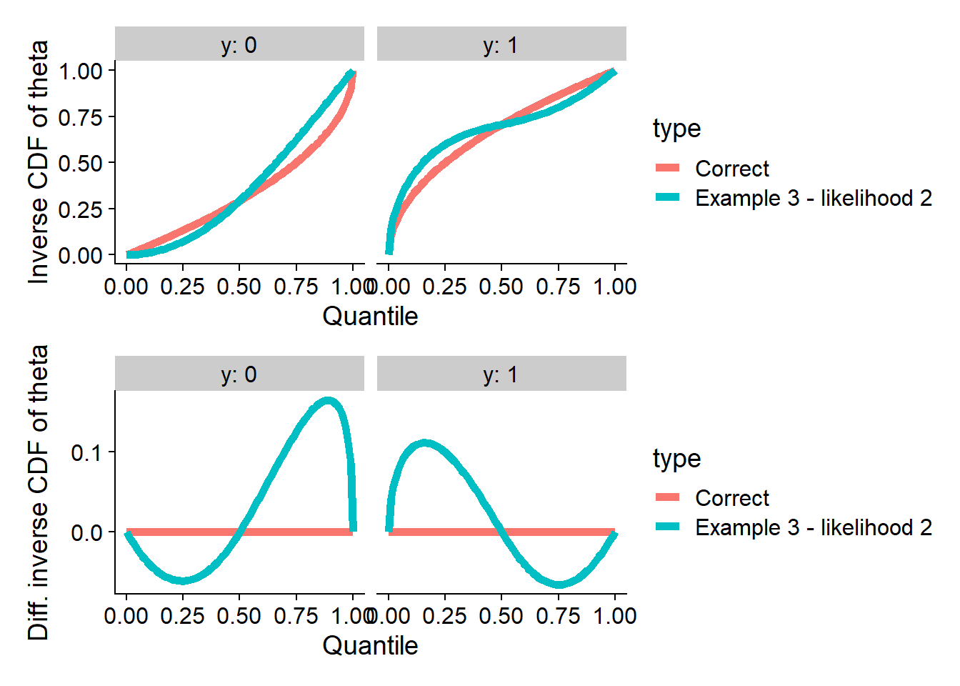

The SBC for both theta and log_lik passes. All the other quantities however do show the failure. This shows the space of useful quantities is not exhausted by a univariate marginal distribution and the (log)likelihood and that non-monotonous transformation of the univariate marginal can provide additional power to SBC.

backend_loglik2 <- my_backend_func_invcdf(invcdf_loglik2_0, invcdf_loglik2_1)

res_loglik2 <- compute_SBC(ds, backend_loglik2, keep_fits = FALSE,
                        dquants = gq_simple, globals = my_globals,
                      cache_mode = "results",
                      cache_location = file.path(cache_dir, "loglik2"))

## Cache file exists but the backend hash differs. Will recompute.

plot_rank_hist(res_loglik2)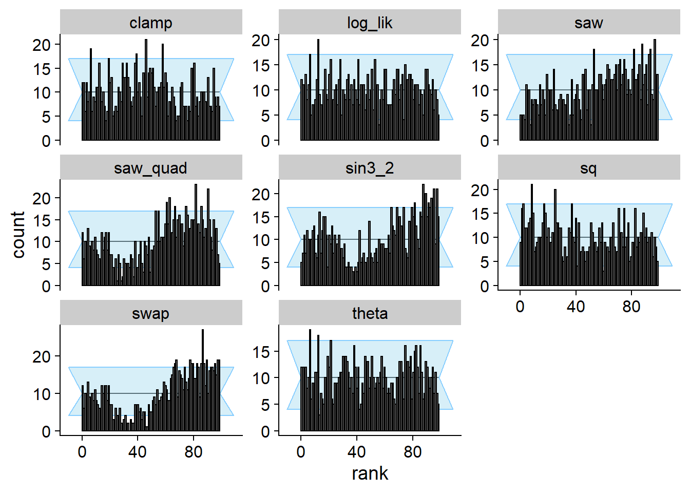

plot_ecdf_diff(res_loglik2)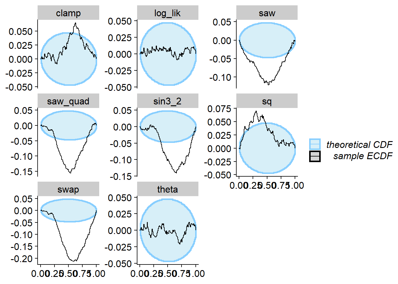

Example 4 - Non-monotonous bijection

Now, we try to build incorrect posterior satisfying SBC for the swap test quantity (called \(f_3\) in the paper). Here, we start once again with \(\Phi^{-1}(x | 0) = x^2\) and then use the formula

$$ ^{-1}(y | 1) = \[\begin{cases} \sqrt{\left(\Phi^{-1}(y + 1 - \bar{h} | 0)\right)^2 - 2 \Phi^{-1}(y + 1 - \bar{h} | 0) + 2(y + 1 - \bar{h} - h_0)} & \text{for } y \leq \bar{h} \\ \sqrt{\left(\Phi^{-1}(y - \bar{h} | 0) - 1 \right)^2 + 2(y - \bar{h} - h_0)} & \text{for } \bar{h} < y \leq 1 + \bar{h} \\ \sqrt{\left( \Phi^{-1}(y - 1 -\bar{h} | 0)\right)^2 - 2 \Phi^{-1}(y - 1 -\bar{h}|0) + 2(y - \bar{h} - h_0)} & \text{for } 1 + \bar{h} < y \\ \end{cases}\]

$$

to create a posterior passing SBC.

invcdf_swap_0 <- function(u) {
  u^2
} 

invcdf_swap_1 <- function(u) {
  h0 <- uniroot(function(x) { invcdf_swap_0(x) - 1/2 }, c(0,1))$root 
  stopifnot(abs(invcdf_swap_0(h0) - 1/2) < 1e-6)
  
  f_h1_larger <- function(h1) {
    #\Phi^{-1}(1 - h_1 + h_0 | 0) = 1 - \sqrt{2h_1 - 1}
    invcdf_swap_0(1 - h1 + h0) - 1 + sqrt(2*h1 - 1)
  }
  f_h1_smaller <- function(h1) {
    #\Phi^{-1}(h_0 - h_1  | 0) = 1 - \sqrt{2h_1}
    invcdf_swap_0(h0 - h1) - 1 + sqrt(2*h1)
  }
  h1_larger_low <- 1/2
  h1_larger_high <- 1 - h0
  h1_smaller_low <- 0
  h1_smaller_high <- h0
  if(h1_larger_low >= h1_larger_high) {
    h1_larger_sign_diff <- FALSE
  } else {
    h1_larger_sign_diff <- sign(f_h1_larger(h1_larger_low)) != sign(f_h1_larger(h1_larger_high))  
  }
  if(h1_smaller_low >= h1_smaller_high) {
    h1_smaller_sign_diff <- FALSE
  } else {
    h1_smaller_sign_diff <- sign(f_h1_smaller(h1_smaller_low)) != sign(f_h1_smaller(h1_smaller_high))  
  }
  
  
  if(h1_larger_sign_diff == h1_smaller_sign_diff) {
    stop("Both sign diffs")
  } else if(h1_larger_sign_diff) {
    h1 <- uniroot(f_h1_larger, c(h1_larger_low,h1_larger_high))$root
  } else {
    h1 <- uniroot(f_h1_smaller, c(h1_smaller_low,h1_smaller_high))$root
  }
  hbar <- h1 - h0
  
  valp1 <- invcdf_swap_0(u + 1 - hbar)
  val0 <- invcdf_swap_0(u - hbar)
  valm1 <- invcdf_swap_0(u - 1 - hbar)
  
  
  
  dplyr::case_when(u < hbar ~ sqrt(valp1^2 - 2 * valp1 + 2 * (u + 1 - hbar - h0)),
            u < 1 + hbar ~ sqrt((val0 - 1)^2 + 2 *( u - hbar - h0)),
            TRUE ~ sqrt(valm1^2 - 2 * valm1 + 2 * (u - hbar - h0))
  )
}

plot_invcdfs(invcdf_swap_0, invcdf_swap_1, "Example 4 - swap")

## Warning in sqrt((val0 - 1)^2 + 2 * (u - hbar - h0)): NaNs produced

## Warning in sqrt(valm1^2 - 2 * valm1 + 2 * (u - hbar - h0)): NaNs produced

## Warning in sqrt((val0 - 1)^2 + 2 * (u - hbar - h0)): NaNs produced

## Warning in sqrt(valm1^2 - 2 * valm1 + 2 * (u - hbar - h0)): NaNs produced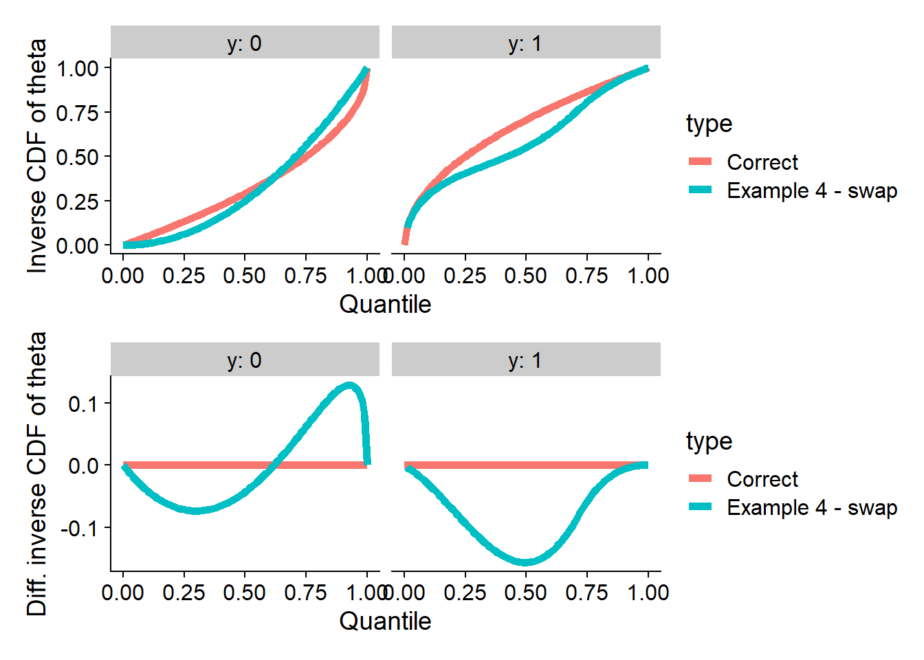

And we run SBC - no problems are seen for swap, while other quantities do show the problem.

backend_swap <- my_backend_func_invcdf(invcdf_swap_0, invcdf_swap_1)

res_swap <- compute_SBC(ds_large, backend_swap, keep_fits = FALSE,
                        dquants = gq_simple, globals = c(my_globals, "invcdf_swap_0"),
                        cache_mode = "results",
                      cache_location = file.path(cache_dir, "swap"))

## Cache file exists but the backend hash differs. Will recompute.

plot_rank_hist(res_swap)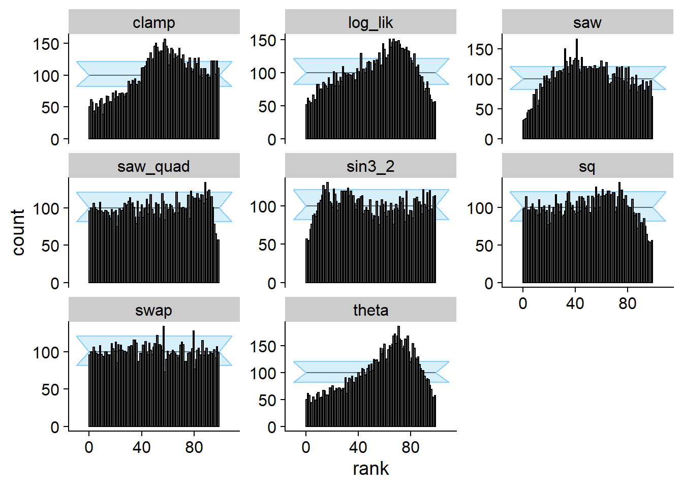

plot_ecdf_diff(res_swap)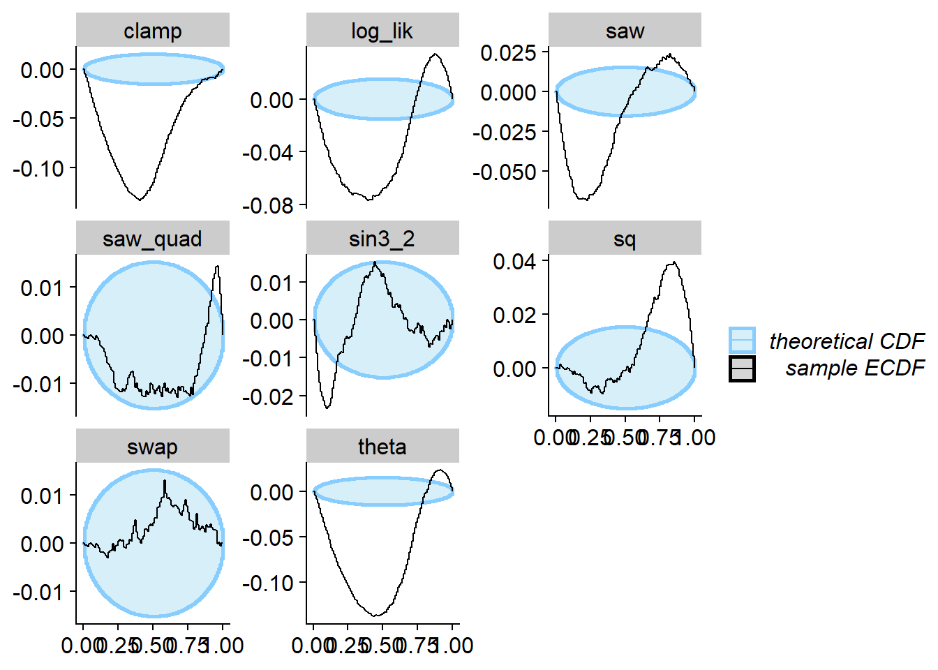

Example 5 - Ties, continuous

Finally, we’ll use what’s called \(f_4\) in the paper and which is called clamp in our plots. That is collapsing a range of values into a single number:

$$ f_4(, y) := \[\begin{cases} \theta & \theta < \frac{1}{2} \\ \frac{1}{2} & \theta \geq \frac{1}{2}. \end{cases}\]

$$

The overall idea is that we can pick \(h_0 = \Phi(\frac{1}{2} | 0)\), compute \(h_1 = \Phi(\frac{1}{2} | 1) = \frac{5 h_0 - 4}{8 h_0 - 7}\) and then \(\Phi^{-1}(x | 0)\) for \(x < \min\{h_0, h_1\}\) quite freely. The problem is that we need to ensure that \(\Phi^{-1}(h_y | y) = \frac{1}{2}\) which introduces some complications - see the paper for details.

Here we take \(\Phi^{-1}(x | 0) = a x^{1.5}\) for \(x < \min\{h_0, h_1\}\) and suitable \(a\).

invcdf_clamp_base <- function() {
  #h0 and basefunc can be +/- freely chosen
  # The basefunc will be appropriately scaled to meet the conditions implied
  # by the choice of h0 (i.e. to ensure invphi(h[y] | y) = 1/2)
  
  # h0 <- 5/8
  # base_func <- function(x) { x }
  h0 <- 0.5
  base_func <- function(x) { x^1.5 }

  stopifnot(h0 < 4/5)

  h1 <- (5*h0 - 4) / (8 *h0 - 7)
  stopifnot( 1/8 < h1 && h1 < 1)
  
  if(h0 < h1) {
    stopifnot(h0 >= 3/8 && h0 < 1/2)
    scale = 0.5 / base_func(h0)
  } else {
    stopifnot(h0 >= 1/2 && h0 < 25/32)
    scale = (1 - 0.5 * sqrt(3/(7 - 8 * h0))) / base_func(h1)
  }
  
  list(
    h0 = h0,
    h1 = h1,
    f =  function(x) { base_func(x) * scale }
  )
}

invcdf_clamp_0 <- function(u) {
  base <- invcdf_clamp_base()
  h0 <- base$h0
  h1 <- base$h1
  
  dplyr::case_when(u <= h0 & u < h1 ~ base$f(u),
            u <= h0 ~ 1 - 0.5 * sqrt((u - 1)/(h0 - 1) ),
            # The value above h0 can be arbitrary as long as it is valid inverse CDF
            # Here we linearly interpolate to 1
            TRUE ~ 0.5 + 0.5 * (u - h0) / (1 - h0))
} 

invcdf_clamp_1 <- function(u) {
  base <- invcdf_clamp_base()
  h0 <- base$h0
  h1 <- base$h1


  val_low <- function(x) {
    sqrt(2 * x  + (base$f(x) - 1 )^2 - 1)
  }
  val_between <- function(x) {
    0.5 * sqrt( ((8 * h0 - 7) * x - 4 * h0 + 3) / (h0 - 1))
  }

  # Check monotonicity
  d <- diff(val_low(seq(0, min(h0, h1), length.out = 200)))
  if(any(is.na(d))) {
    stop("Undefined values for invphi1")
  }
  if(any(d < 0)) {
    stop("Implied invphi1 not increasing")
  }

  dplyr::case_when(u <= h0 & u < h1 ~ val_low(u),
            u <= h1 ~ val_between(u),
            # The value above h1 can be arbitrary as long as it is valid inverse CDF
            # Here we linearly interpolate to 1
            TRUE ~  0.5 + 0.5 * (u - h1) / (1 - h1)
  )
}

plot_invcdfs(invcdf_clamp_0, invcdf_clamp_1, "Example 4 - clamp")

## Warning in sqrt(((8 * h0 - 7) * x - 4 * h0 + 3)/(h0 - 1)): NaNs produced

## Warning in sqrt(((8 * h0 - 7) * x - 4 * h0 + 3)/(h0 - 1)): NaNs produced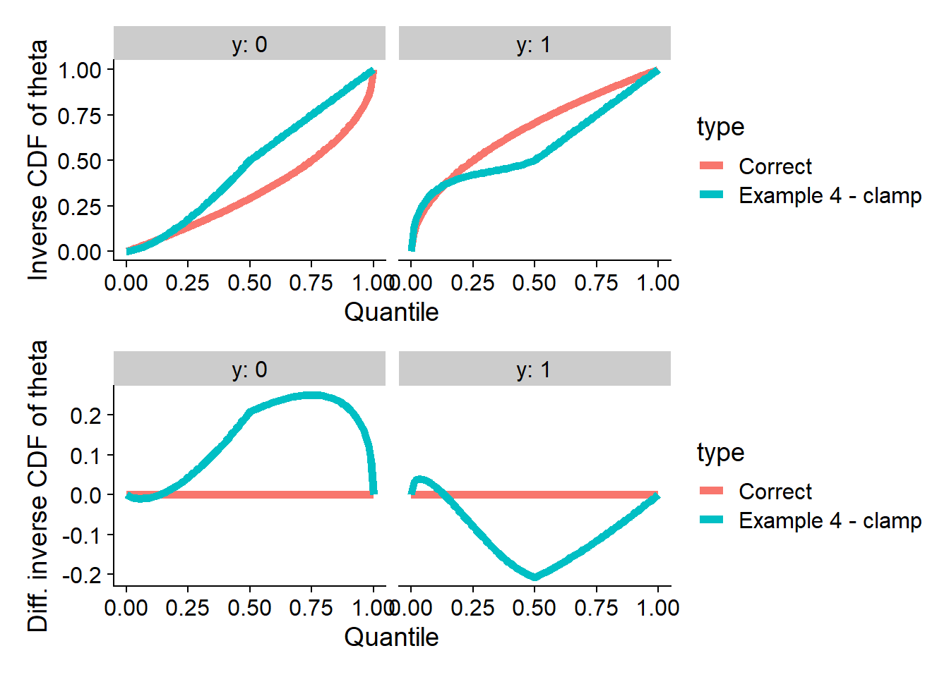

backend_clamp <- my_backend_func_invcdf(invcdf_clamp_0, invcdf_clamp_1)

# We use a bit more datasets to amplify some of the failures
res_clamp <- compute_SBC(ds_large[1:2500], backend_clamp, keep_fits = FALSE,
                        dquants = gq_simple, globals = c(my_globals, "invcdf_clamp_base"),
                        cache_mode = "results",
                      cache_location = file.path(cache_dir, "clamp"))

## Cache file exists but the backend hash differs. Will recompute.

plot_rank_hist(res_clamp)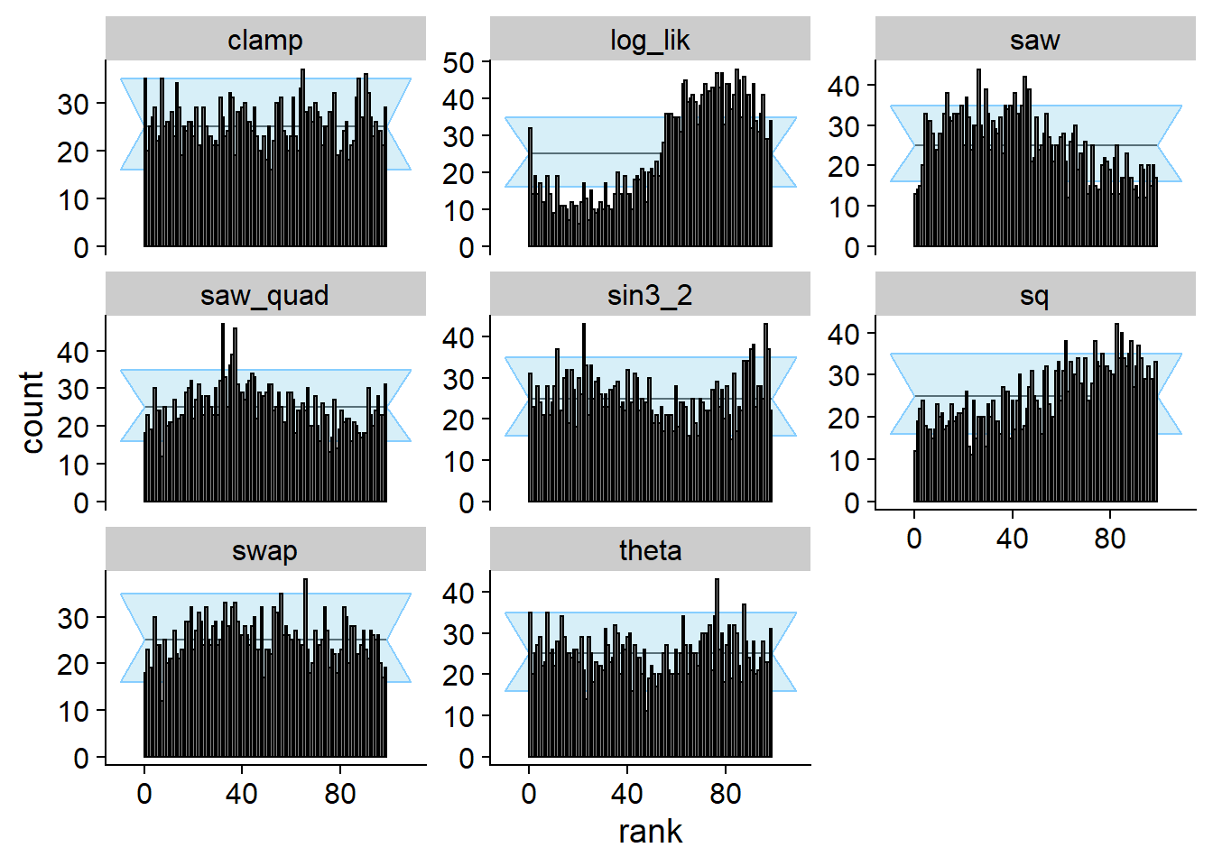

plot_ecdf_diff(res_clamp)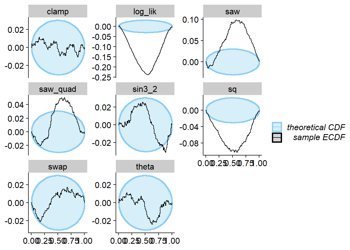

So this posterior passes SBC for clamp and fails for most of the other test quantities. However, recall that almost all of the previous examples failed SBC for clamp.

Additional examples not in the paper

Prior only

Using just the prior as posterior passes SBC for theta and all test quantities that depend only on theta, however the log_lik test quantity comes to the rescue!

backend_prior<- my_backend_func(
  func0 = rlang::as_function(~ runif(N_samples_simple)),
  func1 = rlang::as_function(~ runif(N_samples_simple)))


res_prior <- compute_SBC(ds, backend_prior, keep_fits = FALSE,
                        dquants = gq_simple, globals = my_globals)

plot_rank_hist(res_prior)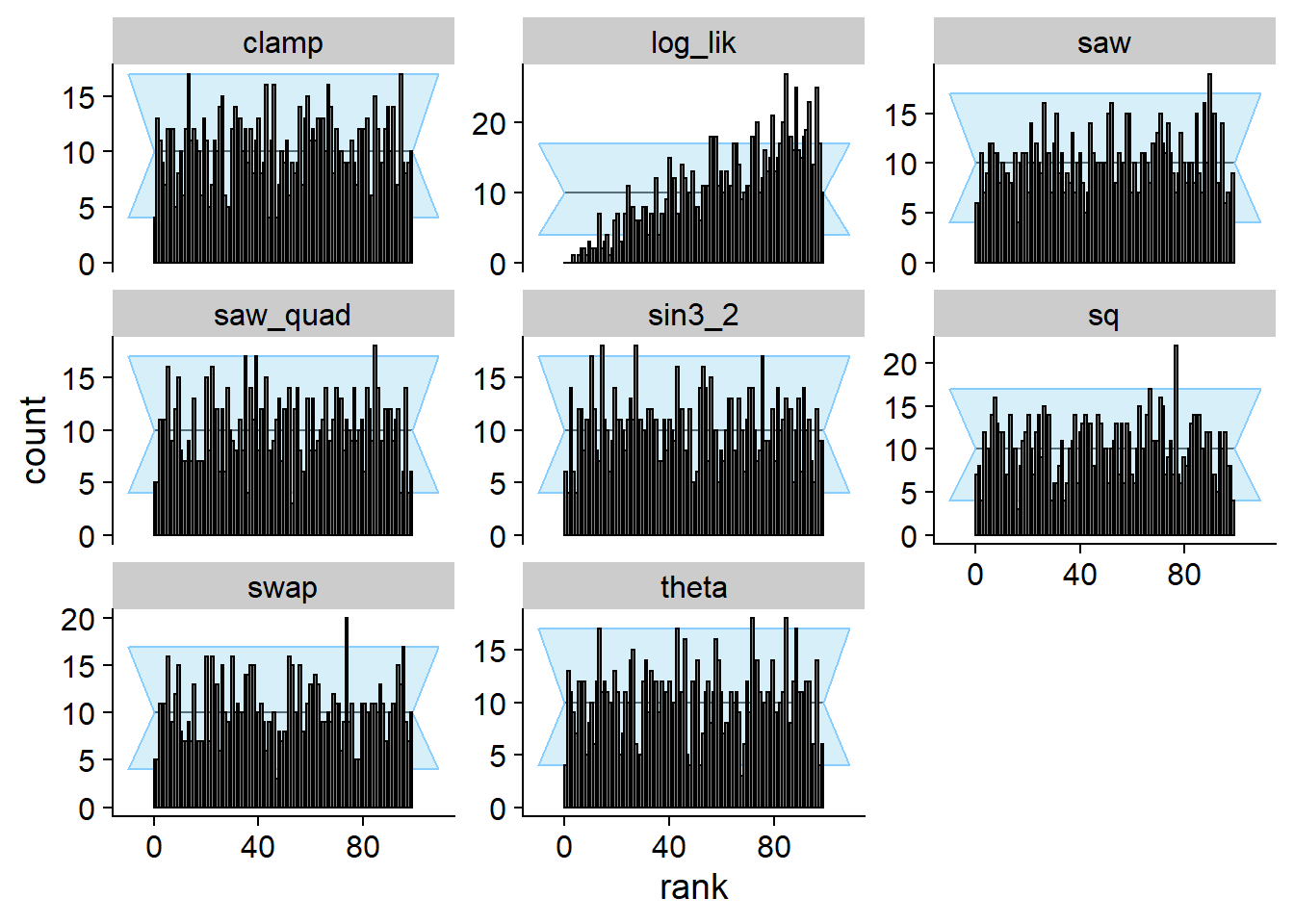

plot_ecdf_diff(res_prior)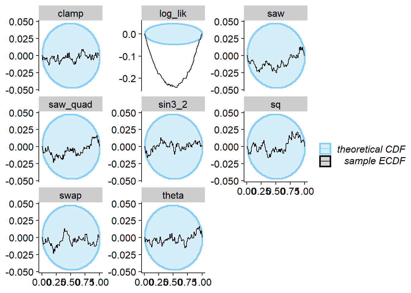

Passing DAP and vanilla SBC

We can in fact build an incorrect posterior that satisfies SBC for projection (theta) and has correct data-averaged posterior. Here is an example:

invcdf_DAP_proj_0 <- function(u) {
  lb = 1/6 * (3 - sqrt(6))
  ub = 1/6 * (3 + sqrt(6))
  ifelse(lb < u & u < ub, 1 - sqrt(11 - 12 * u)/sqrt(12), u)  
} 

invcdf_DAP_proj_1 <- function(u) {
  lb = 1/6 * (3 - sqrt(6))
  ub = 1/6 * (3 + sqrt(6))
  ifelse(lb < u & u < ub, 0.5*sqrt(-1/3 +4* u) , u)  
}

plot_invcdfs(invcdf_DAP_proj_0, invcdf_DAP_proj_1, "Passing SBC and DAP for theta")

## Warning in sqrt(11 - 12 * u): NaNs produced

## Warning in sqrt(-1/3 + 4 * u): NaNs produced

## Warning in sqrt(11 - 12 * u): NaNs produced

## Warning in sqrt(-1/3 + 4 * u): NaNs produced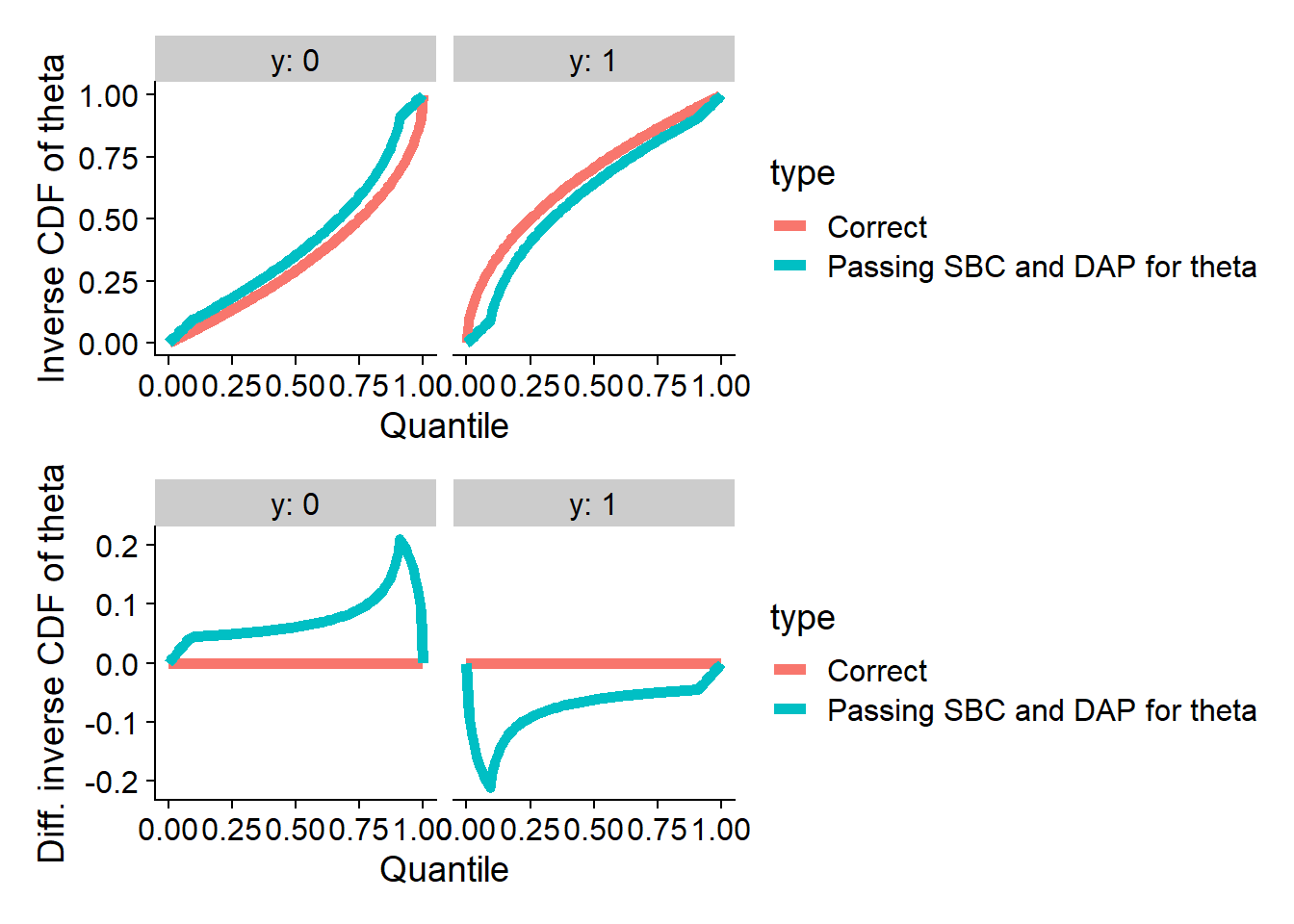

backend_DAP_proj <- my_backend_func_invcdf(invcdf_DAP_proj_0, invcdf_DAP_proj_1)

res_DAP_proj <- compute_SBC(ds_large, backend_DAP_proj, keep_fits = FALSE,
                        dquants = gq_simple, globals = my_globals,
                        cache_mode = "results",
                      cache_location = file.path(cache_dir, "DAP_proj"))

## Cache file exists but the backend hash differs. Will recompute.

plot_rank_hist(res_DAP_proj)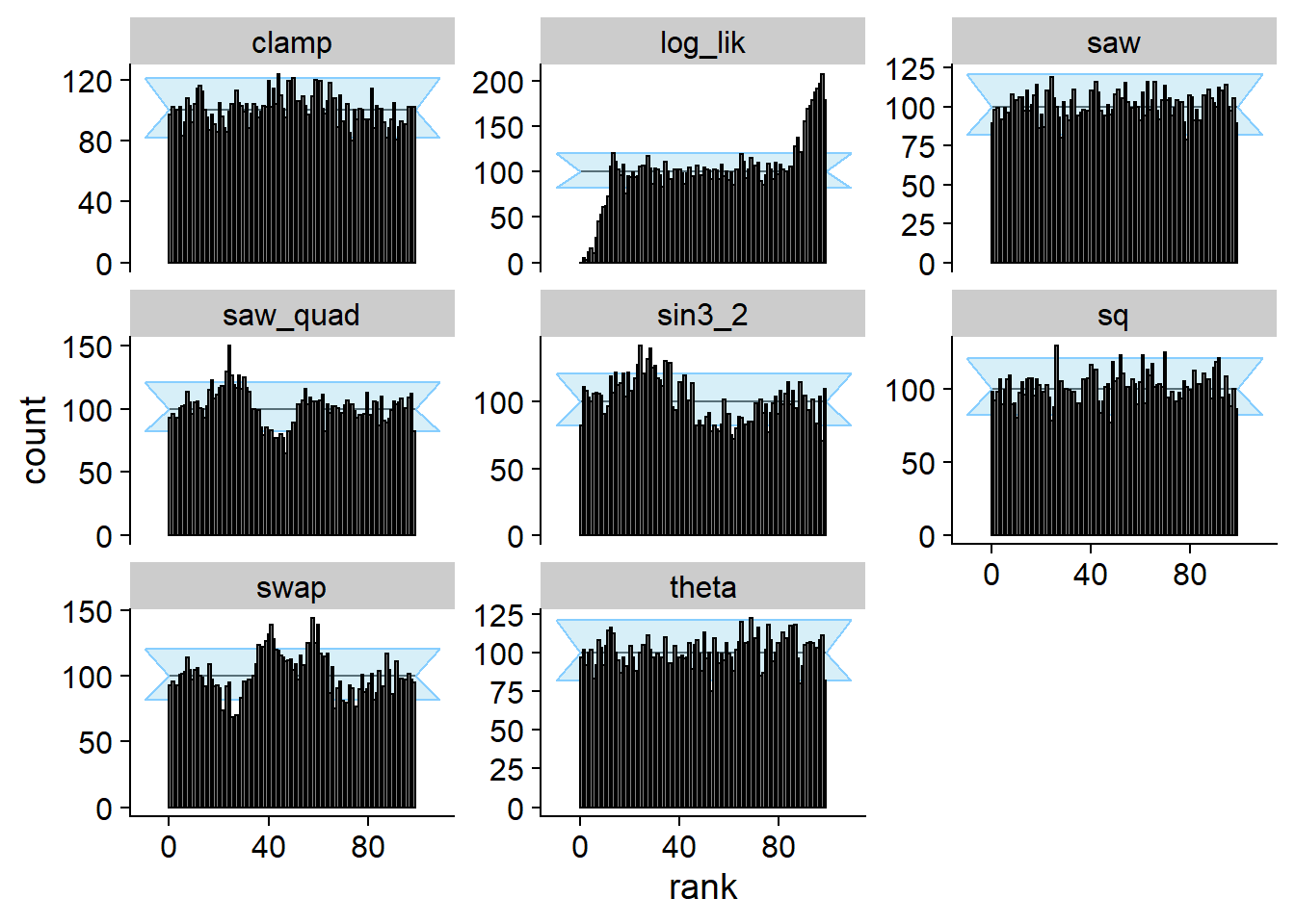

plot_ecdf_diff(res_DAP_proj)