Multivariate normal example

Abstract

This R Markdown document runs the simulations and recreates all the figures used in Section 4 of the paper ‘Simulation-Based Calibration Checking for Bayesian Computation: The Choice of Test Quantities Shapes Sensitivity’

Setting up

The examples are run using the SBC R package. - consult the Getting Started with SBC vignette for basics of the package. We will also use “custom backends” which are discussed and explained in the Implementing a new backend.

knitr::opts_chunk$set(cache = TRUE)
library(SBC)
library(ggplot2)
library(mvtnorm)
library(patchwork)
library(tidyverse)
theme_set(cowplot::theme_cowplot())

options(mc.cores = parallel::detectCores())

library(future)
plan(multisession)

# If true, additional test quantities based on energy score and variogram
# score are included. Those were not very successful and are not discussed
# in the paper.
include_sampling_scores <- FALSE

# Setup caching of SBC results for faster iterations
if(include_sampling_scores) {
  cache_dir <- "./_samp_scores_SBC_cache"
} else {
  cache_dir <- "./_SBC_cache"
}

fig_dir <- "./_figs" 

if(!dir.exists(cache_dir)) {
  dir.create(cache_dir)
}
if(!dir.exists(fig_dir)) {
  dir.create(fig_dir)
}

devtools::load_all()

hist_plot_width <- 8
hist_plot_height <- 3

We are using the model:

\[ \begin{align} \mathbf{\mu} &\sim \mbox{MVN}(0, \mathbf{\Sigma}) \notag \\ \mathbf{y}_1, \ldots, \mathbf{y}_n &\sim \mbox{MVN}(\mathbf{\mu}, \mathbf{\Sigma}) \notag\\ \mathbf{\Sigma} &= \left(\begin{matrix} 1 & 0.8 \\ 0.8 & 1 \\ \end{matrix}\right) \end{align} \]

where \(MVN\) is the multivariate normal distribution. In this case the posterior has analytical solution and should also be multivariate normal.

Now we draw 1000 simulated datasets from this model:

set.seed(266552)

mvn_sigma <- matrix(c(1, 0.8,0.8,1), nrow = 2)

generator_func_correlated <- function(N, sigma = mvn_sigma) {
  mu <- rmvnorm(1, sigma = sigma)
  y <- rmvnorm(N, mean = mu, sigma = sigma)
  list(variables = list(mu = mu[1,]),
       generated = list(y = y))
}

N_sims <- 1000

ds <- generate_datasets(SBC_generator_function(generator_func_correlated, N = 3, sigma = mvn_sigma), N_sims)

We will use a custom backend that will directly generate draws using a function passed into the sampling_func argument.

my_backend_mvn <- function(sampling_func, N_samples = 100, func_extra_args = list()) {
  structure(list(sampling_func = sampling_func, N_samples = N_samples, 
                 func_extra_args = func_extra_args), class = "my_backend_mvn")
}

SBC_fit.my_backend_mvn <- function(backend, generated, cores) {
  all_args <- c(list(y = generated$y, N_samples = backend$N_samples), backend$func_extra_args)
  res_raw <- do.call(backend$sampling_func, all_args)
  
  K <- ncol(generated$y)
  colnames(res_raw) <- paste0("mu[", 1:K, "]")
  posterior::as_draws_matrix(res_raw)
}

SBC_backend_iid_draws.my_backend_mvn <- function(backend) {
  TRUE
}

my_backend_mvn_globals = c("SBC_fit.my_backend_mvn",
                                    "SBC_backend_iid_draws.my_backend_mvn",
                                    "mvn_sigma")

By defualt, SBC will include the individual parameters (mu[1], mu[2]) as test quantities. We now setup the additional test quantities:

quants <- derived_quantities(`mu[1] + mu[2]` = mu[1] + mu[2], 
                               `mu[1] - mu[2]` = mu[1] - mu[2],
                               `mu[1] * mu[2]` = mu[1] * mu[2],
                                mvn_log_lik = sum(mvtnorm::dmvnorm(y, mean = mu, sigma = mvn_sigma, log = TRUE)),
                               `mvn_log_lik[1]` = mvtnorm::dmvnorm(y[1,], mean = mu, sigma = mvn_sigma, log = TRUE),
                               `mvn_log_lik[2]` = mvtnorm::dmvnorm(y[2,], mean = mu, sigma = mvn_sigma, log = TRUE),
                               )

# Ordering the quantities for neat plotting in the paper
order_quants <- function(results) {
  quants_in_order <- c("mu[1]", "mu[2]", 
                    "mu[1] + mu[2]",
                    "mu[1] - mu[2]",
                    "mu[1] * mu[2]",
                     "mvn_log_lik",
                    "mvn_log_lik[1]",
                    "mvn_log_lik[2]",
                    "abs(mu[1])",
                    "drop(mu[1])",
                    "sin(1/mu[1])",
                    "mu[1] * mean(y[,1])",
                    "energy_score",
                    "variogram_score")
  if(!(all(results$stats$variable %in% quants_in_order))) {
    print(setdiff(unique(results$stats$variable, quants_in_order)))
    stop("Unrecognized quants")
  }
  results$stats <- results$stats %>% mutate(variable = factor(variable, levels = quants_in_order))
  results
}

if(include_sampling_scores) {
  sampled_score_mvnorm <- function(y, mu, sigma, score, ...) {
    sim_data <- t(mvtnorm::rmvnorm(200, mean = mu, sigma = sigma))
    res_single <- numeric(nrow(y))
    for(i in 1:nrow(y)) {
      res_single <- score(y[i,], sim_data, ...)
    }
    mean(res_single)
  }
  
  es_mvnorm <- function(y, mu, sigma) {
    sampled_score_mvnorm(y, mu, sigma, scoringRules::es_sample)
  }
  
  vs_mvnorm <- function(y, mu, sigma) {
    sampled_score_mvnorm(y, mu, sigma, scoringRules::vs_sample)
  }
  
  quants_sampled <- derived_quantities(`energy score` = es_mvnorm(y, mu, mvn_sigma),
                               `variogram score` =  vs_mvnorm(y, mu, mvn_sigma),
                               .globals = c("sampled_score_mvnorm", "es_mvnorm", "vs_mvnorm"))
  
  quants <- bind_derived_quantities(quants, quants_sampled)
}

Correct posterior

Introducing \(\bar{\mathbf{y}} = \frac{1}{N}\sum_{i = 1}^{N} \mathbf{y}_i\), the posterior is \(MVN\left(\frac{N\bar{\mathbf{y}}}{n + 1}, \frac{1}{N + 1}\mathbf{\Sigma}\right)\)

Let’s define the sampling function and backend corresponding to the correct posterior and run SBC.

sampling_func_correct <- function(y, N_samples, prior_sigma = mvn_sigma) {
  K <- ncol(y)
  N <- nrow(y)
  
  ybar = colMeans(y)

  post_mean <- N * ybar / (N  + 1)
  post_sigma <- prior_sigma / (N + 1) 
  res_raw <- mvtnorm::rmvnorm(N_samples, mean = post_mean, sigma = post_sigma)
}
backend_correct <- my_backend_mvn(sampling_func_correct)

res_correct <- compute_SBC(ds, backend_correct, dquants = quants, 
                              globals = my_backend_mvn_globals,
                              cache_mode = "results",
                              cache_location = file.path(cache_dir, "mvn_correct"),
                           )

## Cache file exists but the backend hash differs. Will recompute.

res_correct <- order_quants(res_correct)

Those are the diagnostic plots after 1000 simulations.

plot_rank_hist(res_correct)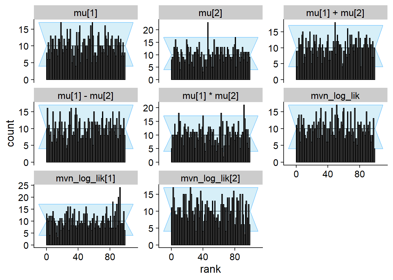

plot_ecdf_diff(res_correct)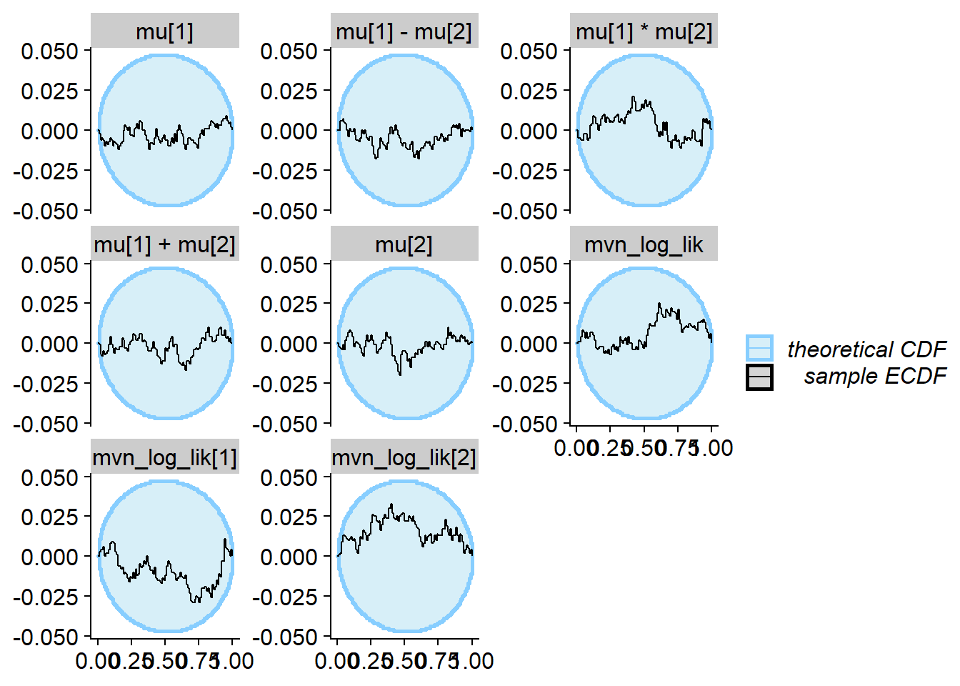

And here is the history of the gamma statistic (see the paper for exact definitons).

p_hist_correct <- plot_log_gamma_history(res_correct)
p_hist_correct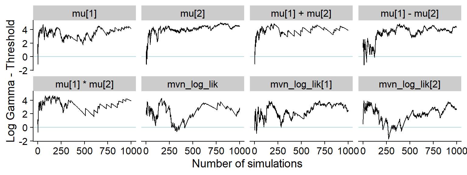

ggsave(file.path(fig_dir, "hist_correct.pdf"), p_hist_correct, width = hist_plot_width, height = hist_plot_height)

For comparison also the history of the p-value for a Kolmogorov-Smirnov test for uniformity (blue horizontal line is 0.05).

plot_ks_test_history(res_correct)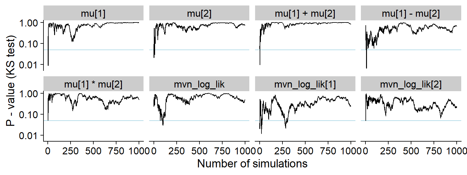

Ignoring Data

Several examples of posteriors that ignore all or some of the data follow.

Prior only

Now we run SBC for a backend that samples from the prior:

sampling_func_prior_only <- function(y, N_samples) {
  mvtnorm::rmvnorm(n = N_samples, sigma = mvn_sigma)
}

backend_prior_only <- my_backend_mvn(sampling_func_prior_only)

res_prior_only <- compute_SBC(ds, backend_prior_only, dquants = quants, 
                              globals = my_backend_mvn_globals,
                              cache_mode = "results",
                              cache_location = file.path(cache_dir, "mvn_prior_only"))

## Cache file exists but the backend hash differs. Will recompute.

res_prior_only <- order_quants(res_prior_only)

Now the diagnostic plots

plot_rank_hist(res_prior_only)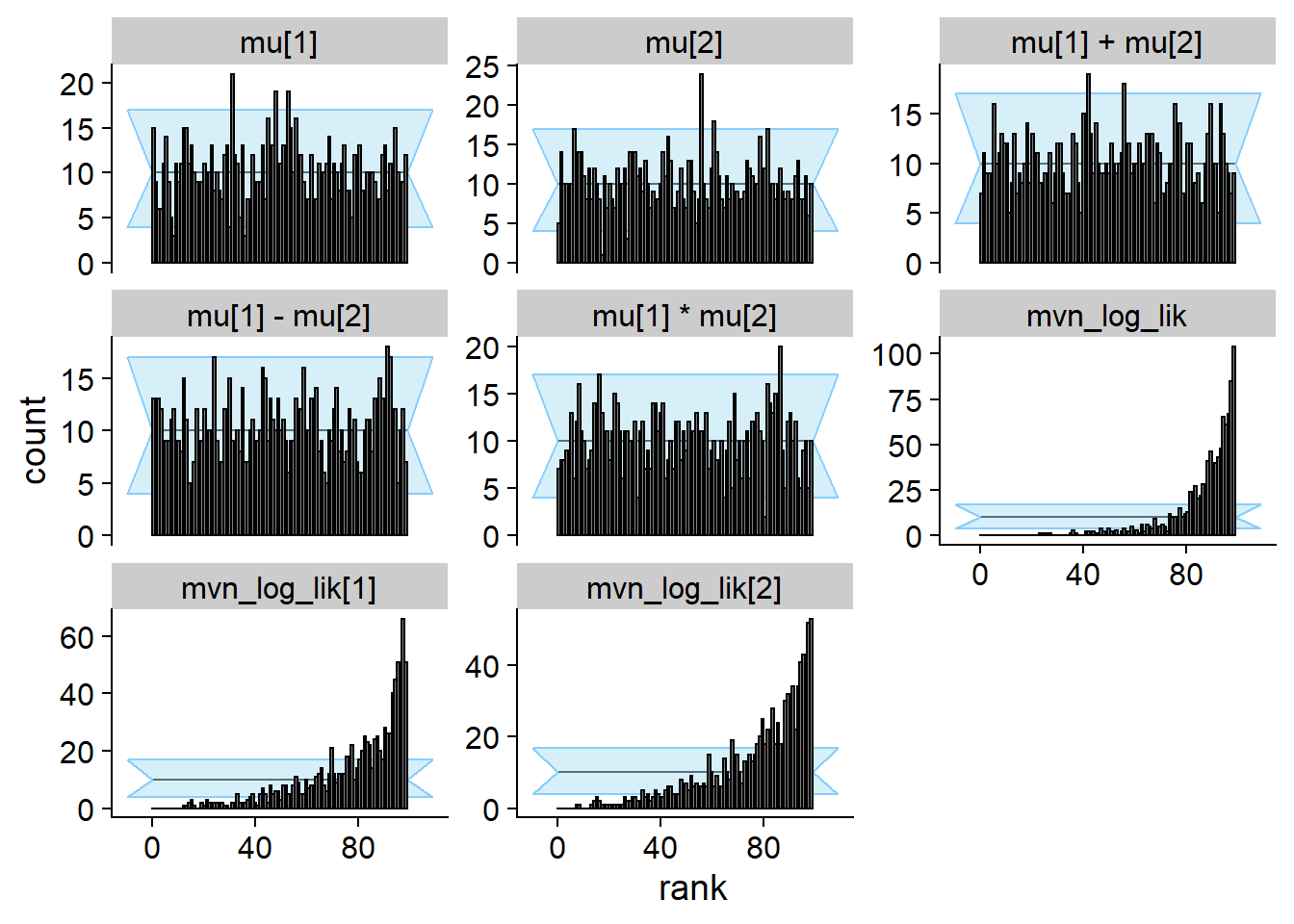

plot_ecdf_diff(res_prior_only)

p_hist_prior_only <- plot_log_gamma_history(res_prior_only, max_sim_id = 50)
p_hist_prior_only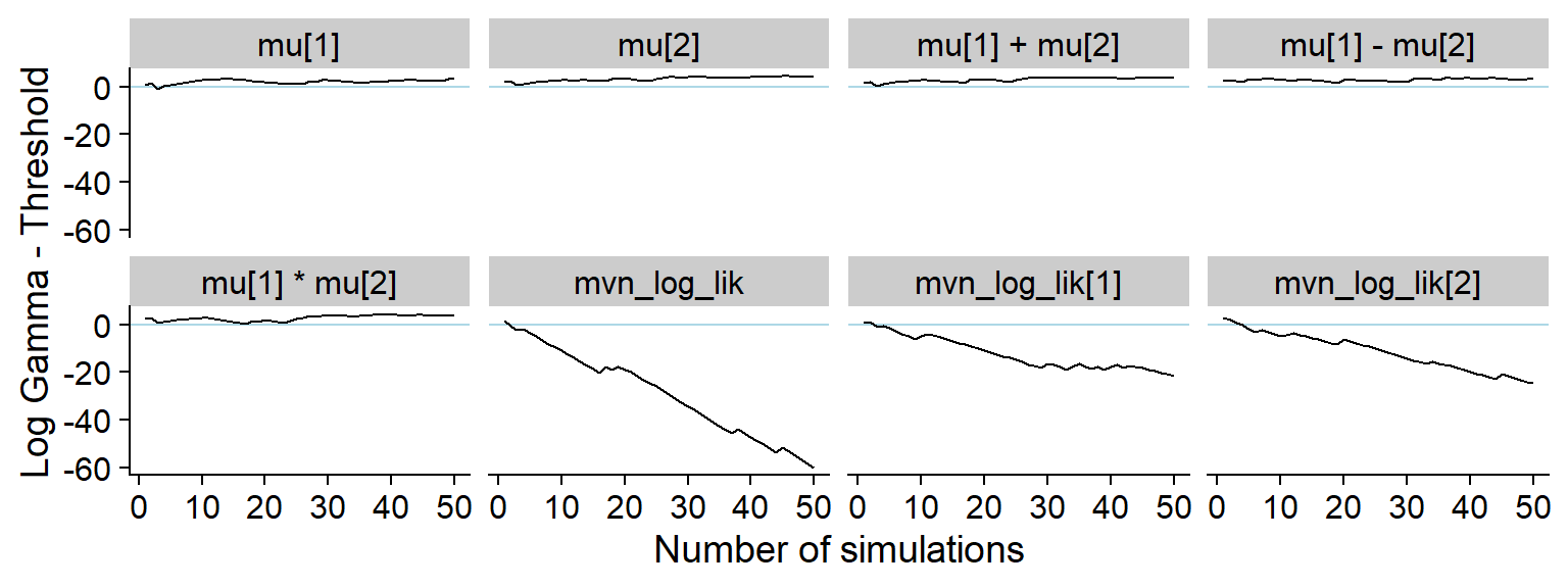

ggsave(file.path(fig_dir, "hist_prior_only.pdf"), p_hist_prior_only, width = hist_plot_width, height = hist_plot_height)

Here’s the rest of the history showing that non-data dependent variables do not show any meaningful discrepancy:

plot_log_gamma_history(res_prior_only, max_sim_id = 1000, variables_regex = "^mu|vario")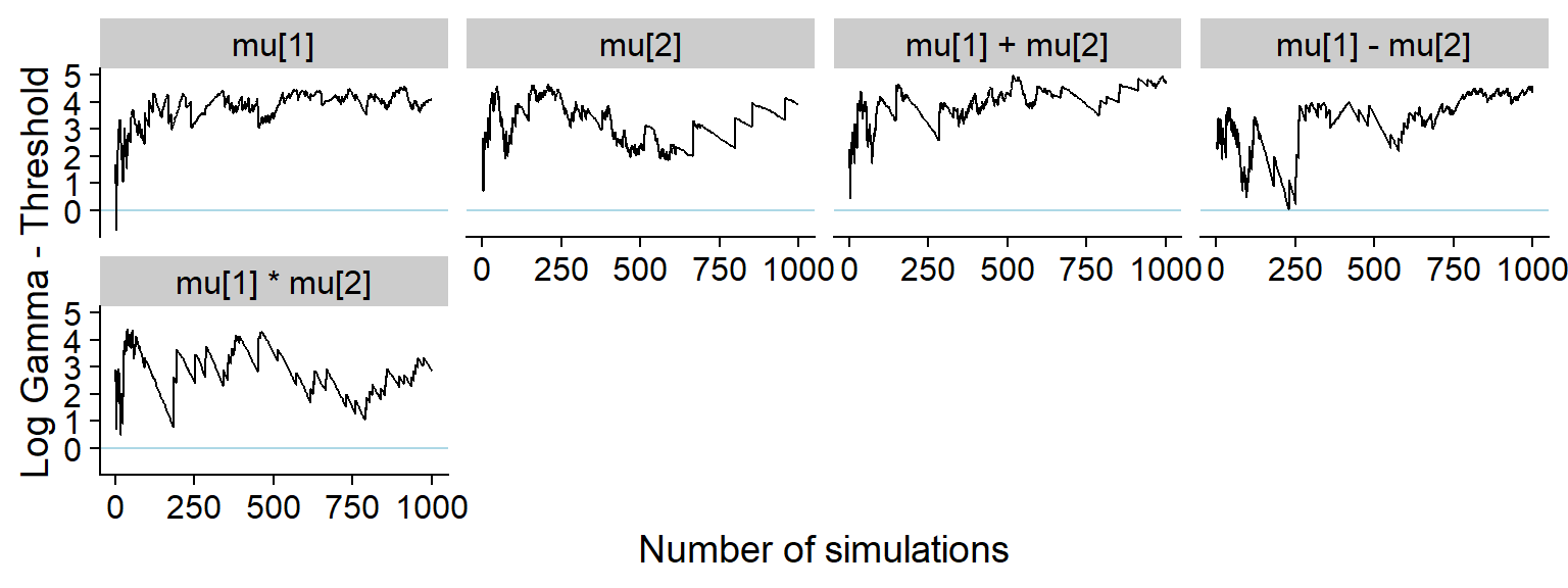

For comparison, here’s the history of the KS p-value:

plot_ks_test_history(res_prior_only, max_sim_id = 50)

## Warning: Transformation introduced infinite values in continuous y-axis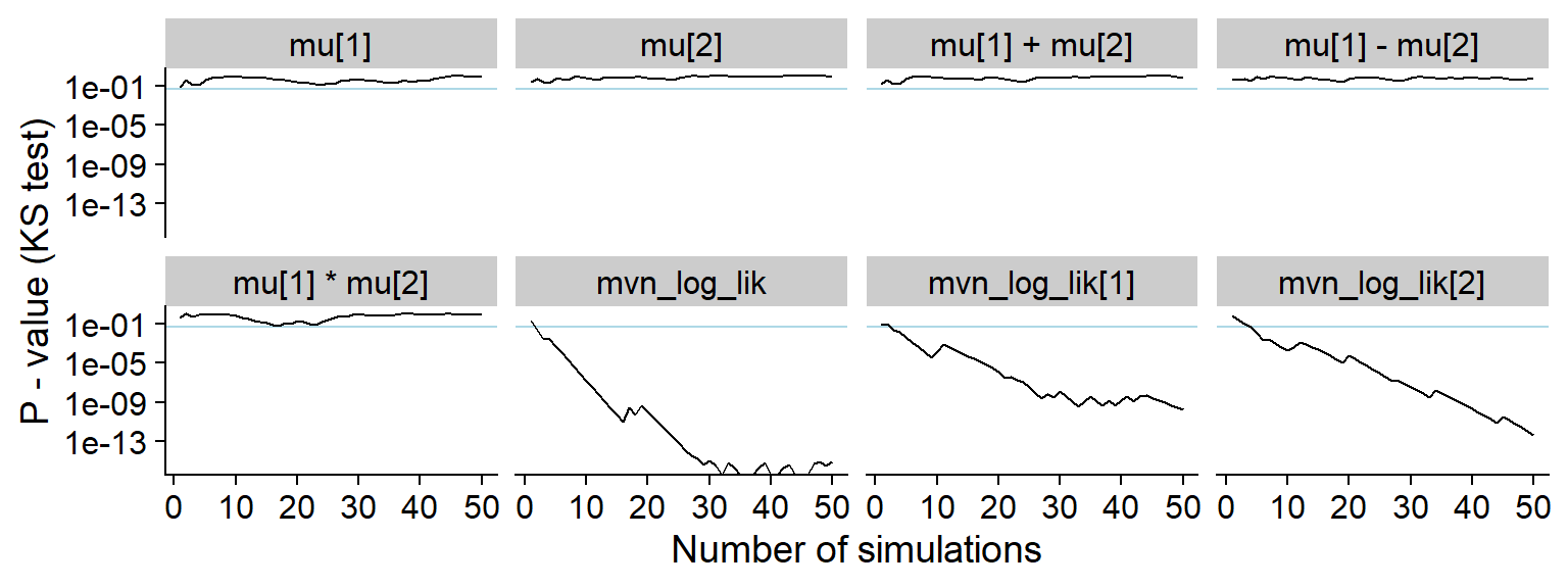

Additonally, we show that splitting the ranks for mu[1] and mu[2] by the average of y results in strongly non-uniform histograms. However the non-uniformity in each subgroup is much smaller than what e.g. the mvn_log_lik quantity provides.

mean1_positive <- which(purrr::map_lgl(ds$generated, function(x) { mean(x$y[,1]) > 0 }))
mean2_positive <- which(purrr::map_lgl(ds$generated, function(x) { mean(x$y[,2]) > 0 }))
stats_split <- res_prior_only$stats %>% filter(variable %in% c("mu[1]", "mu[2]")) %>%
  mutate(variable = paste0(variable, " - mean y ", 
                           if_else(if_else(variable == "mu[1]", sim_id %in% mean1_positive, sim_id %in% mean2_positive), 
                                   "positive", "negative"))
                            )

# The visualisations in SBC package do not supprt different variables have different
# number of simulations. We thus discard simulations to keep both groups of the same size.
min_n <- stats_split %>% group_by(variable) %>% summarise(n = n()) %>% pull(n) %>% min()

stats_split <- stats_split %>% group_by(variable) %>%
  mutate(sim_id = 1:n()) %>%
  ungroup() %>%
  filter(sim_id <= min_n)

p_rank_hist_prior_only_split <- plot_rank_hist(stats_split) + facet_wrap(~variable, nrow = 1)
p_rank_hist_prior_only_split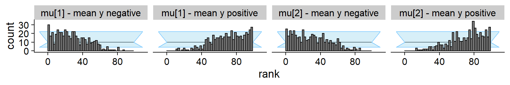

ggsave(file.path(fig_dir, "rank_hist_prior_only_split.pdf"), p_rank_hist_prior_only_split, width = hist_plot_width + 1, height = hist_plot_height / 2 )

One missing data point

Now we have one data point missing:

sampling_func_one_missing <- function(y, N_samples) {
  # Delegate to the correct posterior, just throw away data
  sampling_func_correct(y[2:nrow(y),], N_samples)
}

backend_one_missing <- my_backend_mvn(sampling_func_one_missing)

set.seed(5652265)
res_one_missing <- compute_SBC(ds, backend_one_missing, dquants = quants, 
                              globals = c(my_backend_mvn_globals, "sampling_func_correct"),
                              cache_mode = "results",
                              cache_location = file.path(cache_dir, "mvn_one_missing"))

## Cache file exists but the backend hash differs. Will recompute.

res_one_missing <- order_quants(res_one_missing)

The diagnostic plots:

plot_rank_hist(res_one_missing)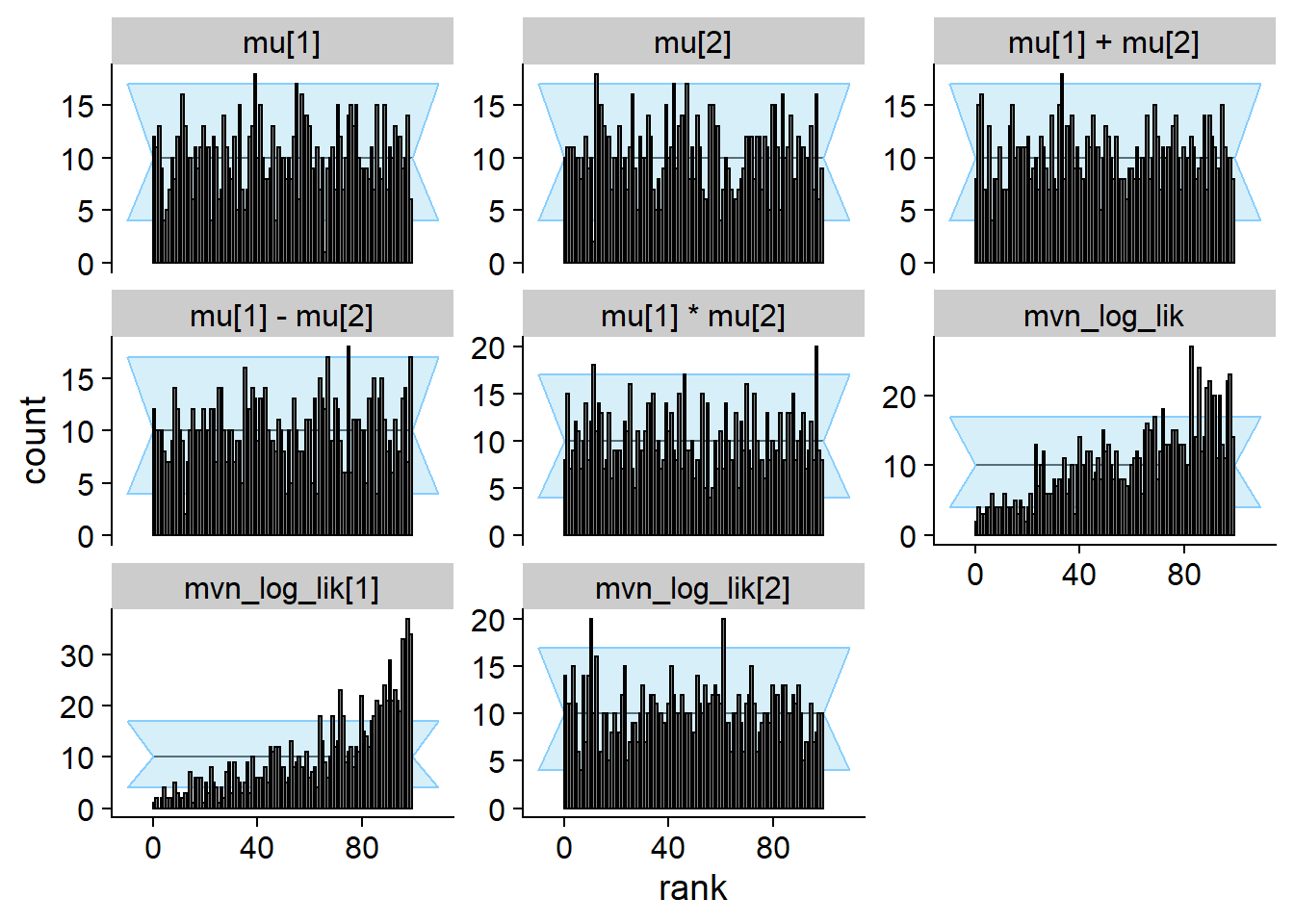

plot_ecdf_diff(res_one_missing)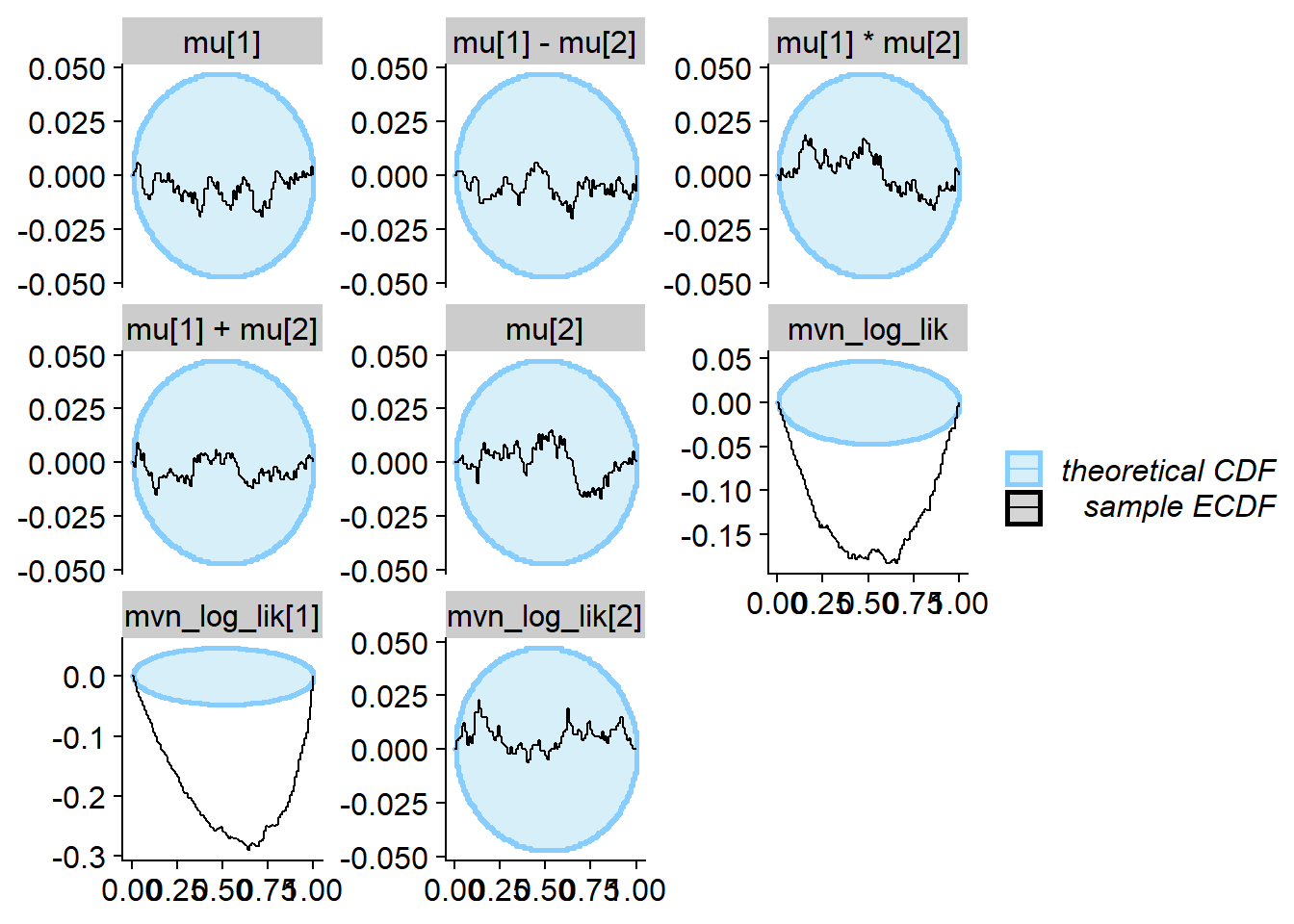

And the history of the gamma statistic

p_hist_one_missing <- plot_log_gamma_history(res_one_missing, max_sim_id = 100)
p_hist_one_missing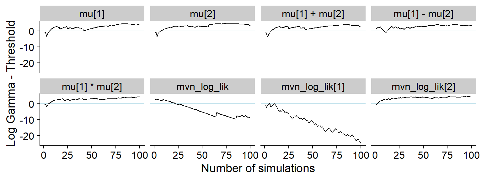

ggsave(file.path(fig_dir, "hist_one_missing.pdf"), p_hist_one_missing, width = hist_plot_width, height = hist_plot_height)

A bit longer window

plot_log_gamma_history(res_one_missing, max_sim_id = 500)

And the KS p-value - note that the initial discrepancies in all of the quantities look more serious in this view (although the non-likelihood quantities in fact have uniform distribution)

plot_ks_test_history(res_one_missing, max_sim_id = 500)

## Warning: Transformation introduced infinite values in continuous y-axis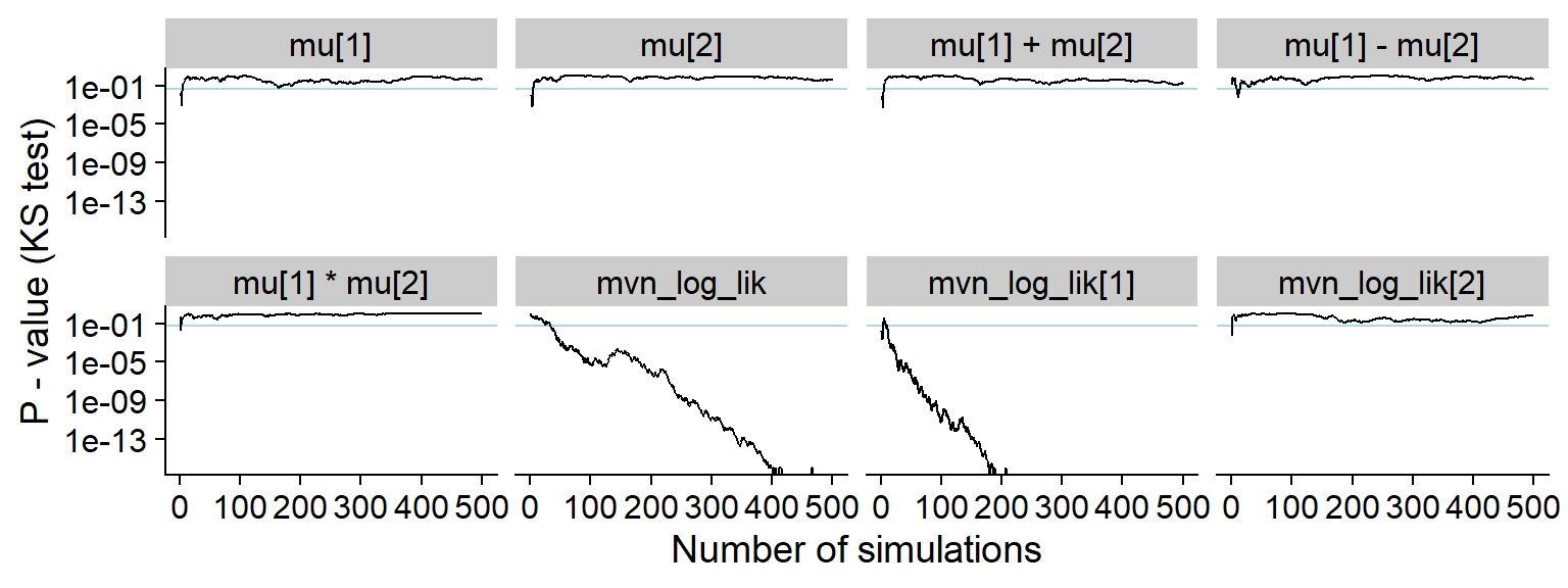

One missing data point - larger N

Identical setup as above, but we have 20 data points.

# Generate datasets with 20 datapoints.
set.seed(2665884)
ds_20 <- generate_datasets(SBC_generator_function(generator_func_correlated, N = 20, sigma = mvn_sigma), N_sims)


res_one_missing_20 <- compute_SBC(ds_20, backend_one_missing, dquants = quants, 
                              globals = c(my_backend_mvn_globals, "sampling_func_correct"),
                              cache_mode = "results",
                              cache_location = file.path(cache_dir, "mvn_one_missing_20"))

## Cache file exists but the backend hash differs. Will recompute.

res_one_missing_20 <- order_quants(res_one_missing_20)

The final diagnostic plots

plot_rank_hist(res_one_missing_20)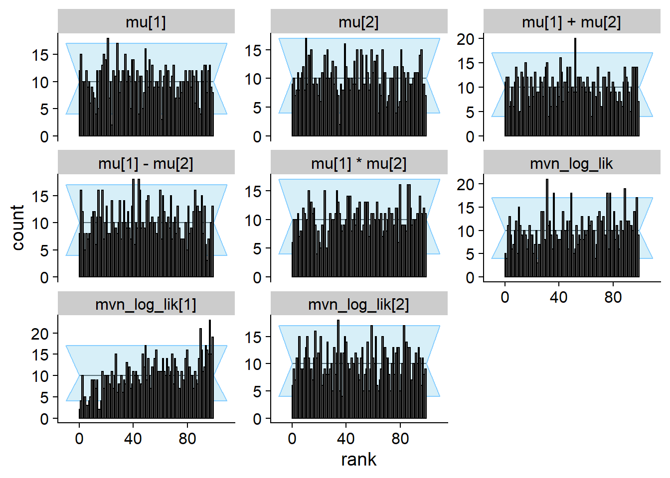

plot_ecdf_diff(res_one_missing_20)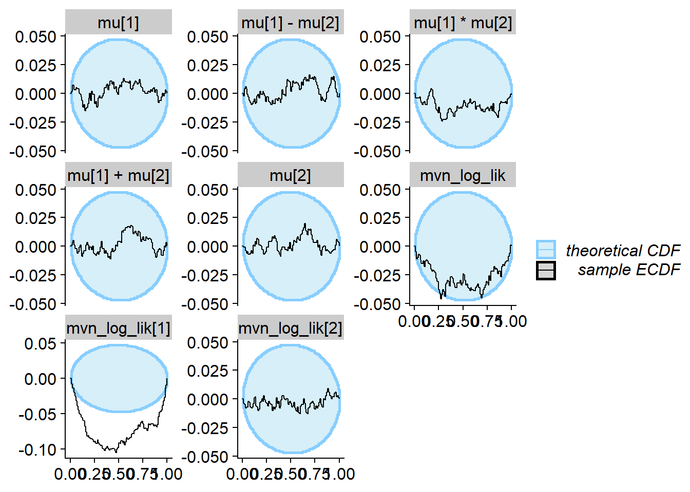

History of gamma statistic

p_hist_one_missing_20 <- plot_log_gamma_history(res_one_missing_20)
p_hist_one_missing_20

ggsave(file.path(fig_dir, "hist_one_missing_20.pdf"), p_hist_one_missing_20, width = hist_plot_width, height = hist_plot_height)

History of KS p-value

plot_ks_test_history(res_one_missing_20)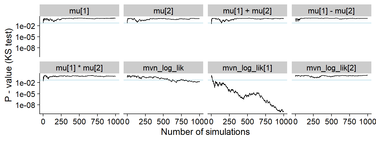

Incorrect posterior correlations

Especially when the number of data points is small, the correlations in the prior should persist in the posterior.

We however generate posterior samples from a set of independent normal distributions that happen to have the correct mean and standard deviation, just the correlation is missing.

sampling_func_uncorr <- function(y, N_samples, prior_sigma = 1) {
  K <- ncol(y)
  N <- nrow(y)
  
  ybar = colMeans(y)

  res_raw <- matrix(nrow = N_samples, ncol = K)
  for(k in 1:K) {
    post_mean <- N * ybar[k] / (N  + 1)
    post_sd <- sqrt(1 / (N + 1)) * prior_sigma 
    res_raw[,k] <- rnorm(N_samples, mean = post_mean, sd = post_sd)
  }
  res_raw
}

backend_uncorr <- my_backend_mvn(sampling_func_uncorr)


res_uncorr <- compute_SBC(ds, backend_uncorr, 
                        globals = my_backend_mvn_globals,
                        dquants = quants,
                        cache_mode = "results", 
                        cache_location = file.path(cache_dir, "mvn_uncorr"))

## Cache file exists but the backend hash differs. Will recompute.

res_uncorr <- order_quants(res_uncorr)

Although the posterior is incorrect, the default univariate checks don’t show any problem even with 1000 simulations. All of the other quantities however show issues.

plot_rank_hist(res_uncorr)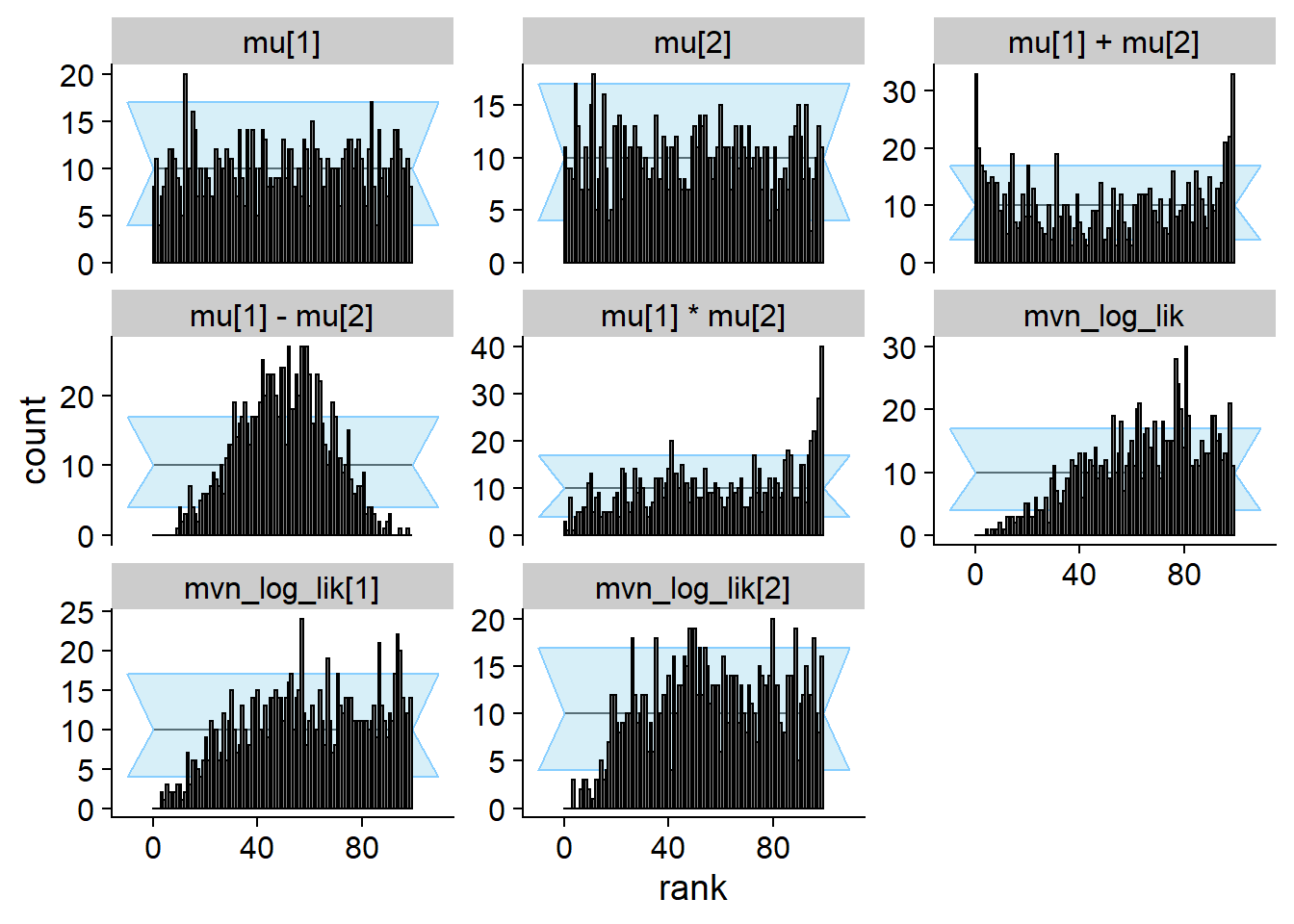

plot_ecdf_diff(res_uncorr)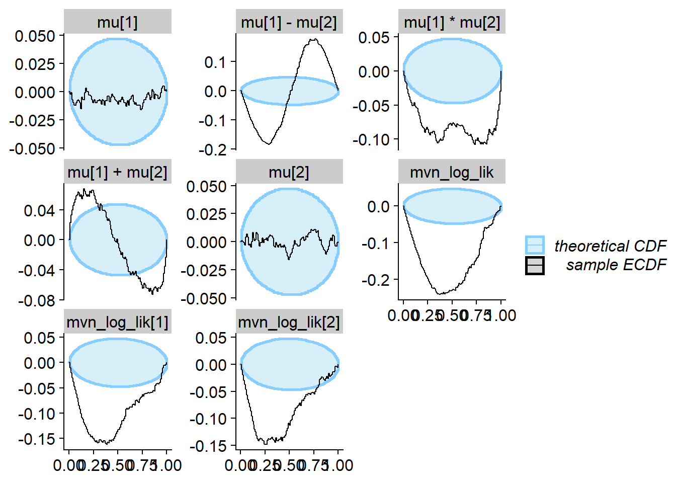

The history of the gamma statistic.

p_hist_corr <- plot_log_gamma_history(res_uncorr, max_sim_id = 100)
p_hist_corr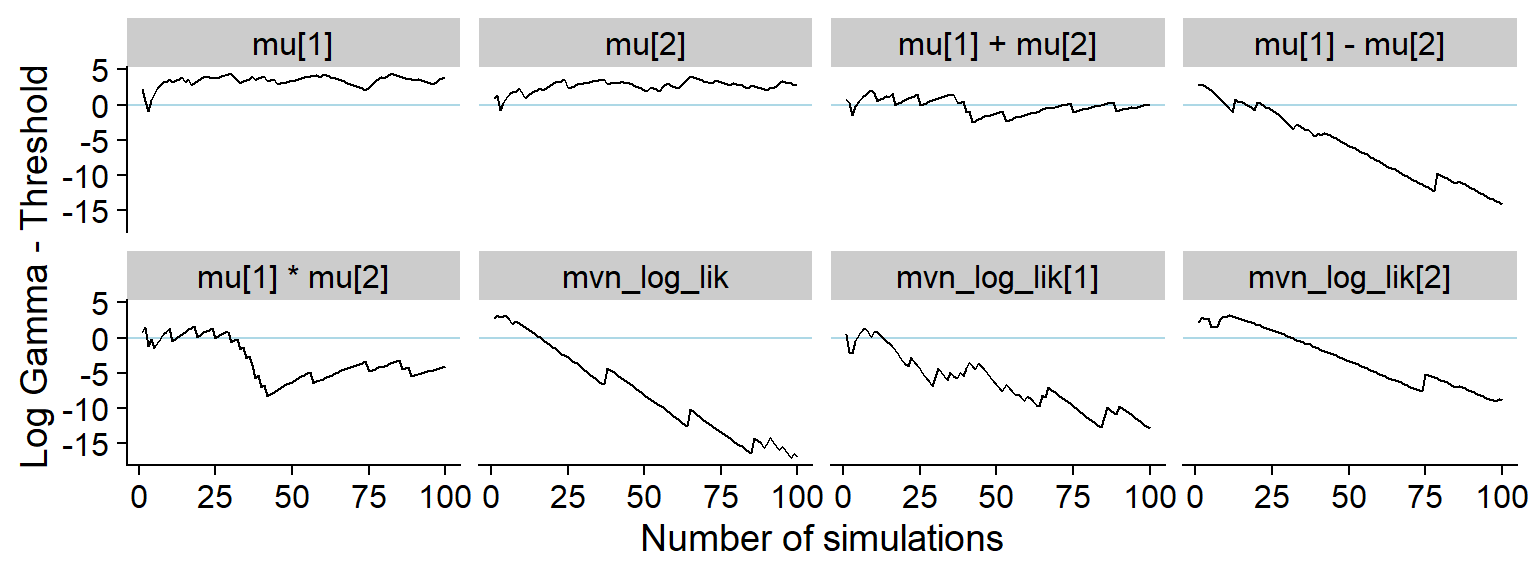

ggsave(file.path(fig_dir, "hist_corr.pdf"), p_hist_corr, width = hist_plot_width, height = hist_plot_height)

A somewhat longer window shows how all the quantities produce issues:

plot_log_gamma_history(res_uncorr, max_sim_id = 250)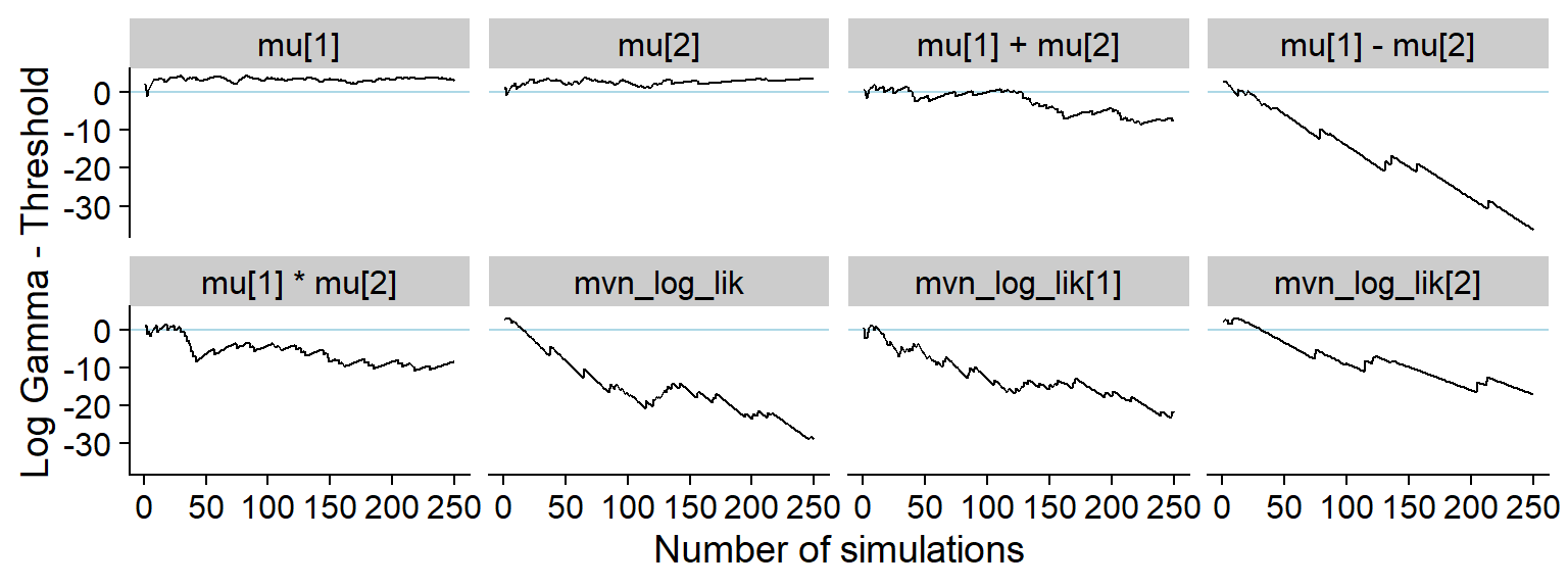

And KS p-value. Note the lowered sensitivity towards issues with mu[1] * mu[2] and mu[1] + mu[2].

plot_ks_test_history(res_uncorr, max_sim_id = 250)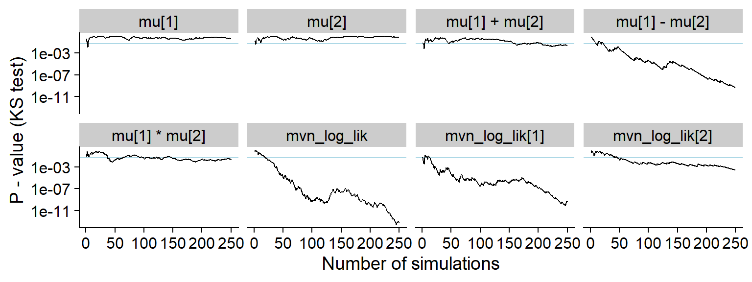

Non-monotonous transform

Finally our backend showing the (probably not very practical) utility of non-monotonous transformations.

set.seed(246855)
# Generate even more datasets - same quantities take loooong to show problems
ds_more <- bind_datasets(
  ds,
  generate_datasets(SBC_generator_function(generator_func_correlated, N = 3, sigma = mvn_sigma), n_sims = 5000)
)

Now let us build the sampling function. The overall idea is that we start with the correct posterior. We then use the CDF to transform the samples to [0,1], manipulate the value on this scale to achieve the desired CDF shape and than transform back with the quantile function.

sampling_func_non_mon <- function(y, N_samples, prior_sigma = mvn_sigma) {
  # Sample as if correct
  K <- ncol(y)
  N <- nrow(y)
  
  ybar = colMeans(y)

  post_mean <- N * ybar / (N  + 1)
  post_sigma <- prior_sigma / (N + 1) 
  res <- mvtnorm::rmvnorm(N_samples, mean = post_mean, sigma = post_sigma)

  # Modify
  for(k in 1:K) {
    res_k <- res[,k]
    
    uniform_q <- pnorm(res_k, post_mean[k], sqrt(post_sigma[k,k]))
    if(mean(y[,k]) > 0) {
      transformed_q <- dplyr::if_else(uniform_q < 0.5, 1.5 * uniform_q, 0.75 + (uniform_q - 0.5)*0.5)
    } else {
      transformed_q <- dplyr::if_else(uniform_q < 0.5, 0.5 * uniform_q, 0.25 + (uniform_q - 0.5)*1.5)
    }
    res_k <- qnorm(transformed_q, post_mean[k], sqrt(post_sigma[k,k]))
    
    res[,k] <- res_k
  }
  res
}

backend_non_mon <- my_backend_mvn(sampling_func_non_mon)

# Define different test quantities
quants_non_mon <- derived_quantities(`mu[1] * mu[2]` = mu[1] * mu[2],
                                       `abs(mu[1])` = abs(mu[1]),
                                       `drop(mu[1])` = ifelse(mu[1] < 1, mu[1], mu[1] - 5),
                                       `sin(1/mu[1])` = sin(1/mu[1]),
                                       `mu[1] * mean(y[,1])` = mu[1] * mean(y[,1]),
                                mvn_log_lik = sum(mvtnorm::dmvnorm(y, mean = mu, sigma = mvn_sigma, log = TRUE)))

if(include_sampling_scores) {
  quants_non_mon <- bind_derived_quantities(quants_non_mon, quants_sampled)
}



  
res_non_mon <- compute_SBC(ds_more, backend_non_mon, dquants = quants_non_mon, 
                              globals = c(my_backend_mvn_globals, "sampling_func_correct"),
                              cache_mode = "results",
                              cache_location = file.path(cache_dir, "mvn_non_mon"))

## Cache file exists but the backend hash differs. Will recompute.

res_non_mon <- order_quants(res_non_mon)

The diagnostic plots

plot_rank_hist(res_non_mon)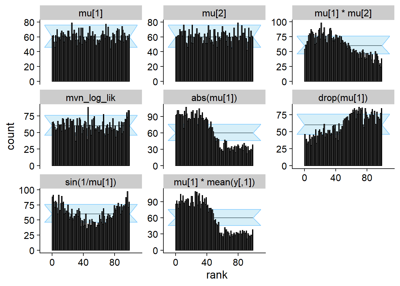

plot_ecdf_diff(res_non_mon)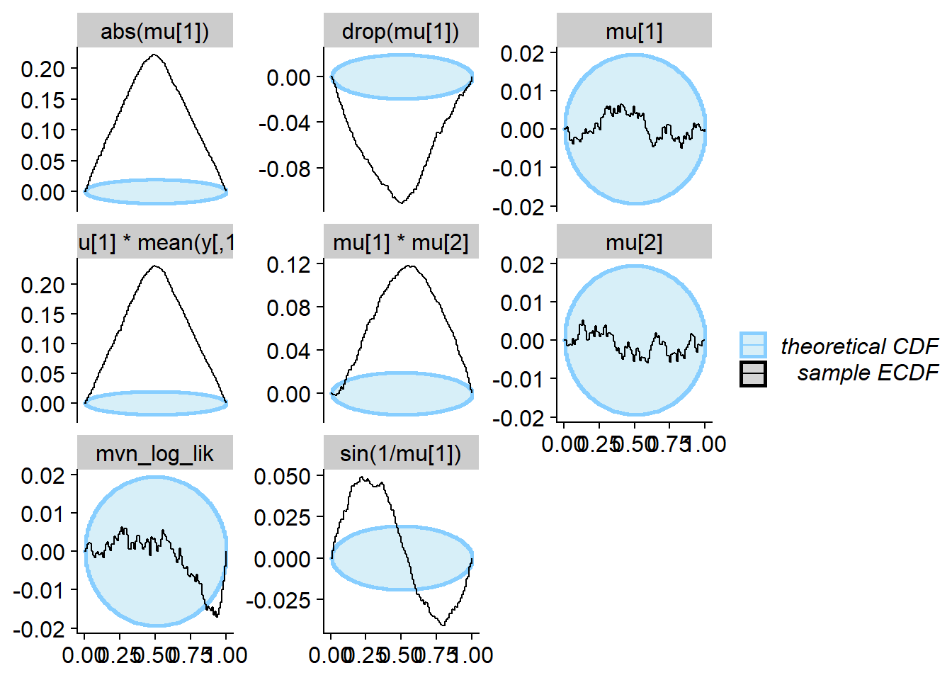

Show that the manipulation of the ranks was succesful - those are the ranks split by positive/negative mean of y.

mean1_positive <- which(purrr::map_lgl(ds_more$generated, function(x) { mean(x$y[,1]) > 0 }))
mean2_positive <- which(purrr::map_lgl(ds_more$generated, function(x) { mean(x$y[,2]) > 0 }))
stats_split <- res_non_mon$stats %>% filter(variable %in% c("mu[1]", "mu[2]")) %>%
  mutate(variable = paste0(variable, " - mean y ", 
                           if_else(if_else(variable == "mu[1]", sim_id %in% mean1_positive, sim_id %in% mean2_positive), 
                                   "positive", "negative"))
                            )
# The visualisations in SBC package do not supprt different variables have different
# number of simulations. We thus discard simulations to keep both groups of the same size.
min_n <- stats_split %>% group_by(variable) %>% summarise(n = n()) %>% pull(n) %>% min()

stats_split <- stats_split %>% group_by(variable) %>%
  mutate(sim_id = 1:n()) %>%
  ungroup() %>%
  filter(sim_id <= min_n)

p_rank_hist_non_mon_split <- plot_rank_hist(stats_split) + facet_wrap(~variable, nrow = 1)
p_rank_hist_non_mon_split

ggsave(file.path(fig_dir, "rank_hist_non_mon_split.pdf"), p_rank_hist_non_mon_split, width = hist_plot_width + 1, height = hist_plot_height / 2 )

Now the history. To make everything well visible, show only a subset of the simulations for some quantities:

shared_mark <- geom_vline(color = "red", linetype = "dashed", xintercept = 500)
p_hist_non_mon_1 <- plot_log_gamma_history(res_non_mon, ylim = c(-30, 5), variables_regex = "(^mu\\[.\\]$)|lik|sin") + 
  theme(axis.title = element_blank()) + shared_mark
p_hist_non_mon_2 <- plot_log_gamma_history(res_non_mon, ylim = c(-30, 5), max_sim_id = 500, variables_regex = "abs|\\*|drop") +
  theme(axis.title = element_blank()) + shared_mark

#axis title: https://stackoverflow.com/questions/65291723/merging-two-y-axes-titles-in-patchwork
p_label <- ggplot(data.frame(l = "Log Gamma - Threshold", x = 1, y = 1)) +
      geom_text(aes(x, y, label = l), angle = 90, size = 5) + 
      theme_void() +
      coord_cartesian(clip = "off")

p_hist_non_mon <- p_label + (p_hist_non_mon_1 / p_hist_non_mon_2) + plot_layout(widths = c(0.4, 25))
p_hist_non_mon

## Warning: Removed 676 row(s) containing missing values (geom_path).

## Warning: Removed 252 row(s) containing missing values (geom_path).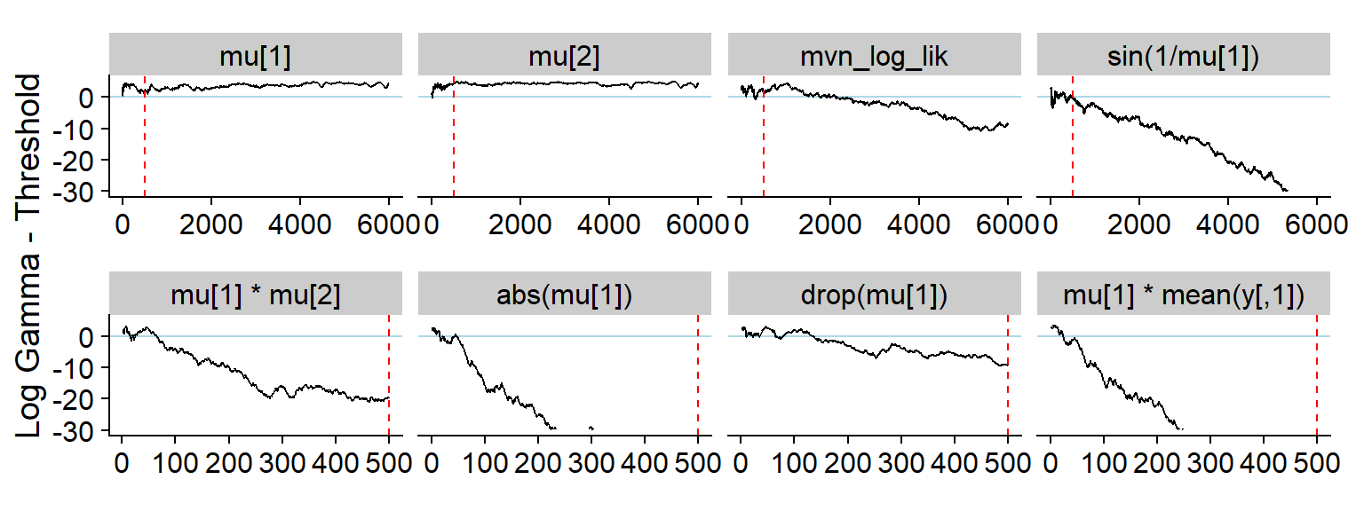

ggsave(file.path(fig_dir, "hist_non_mon.pdf"), p_hist_non_mon, width = hist_plot_width, height = hist_plot_height)

## Warning: Removed 676 row(s) containing missing values (geom_path).
## Removed 252 row(s) containing missing values (geom_path).

This is the history without any modifications. Note that for several quantities the values crash too low and become NaN.

p_hist_non_mon_ext <- plot_log_gamma_history(res_non_mon, ylim = c(-30, 5))
p_hist_non_mon_ext

## Warning: Removed 5752 row(s) containing missing values (geom_path).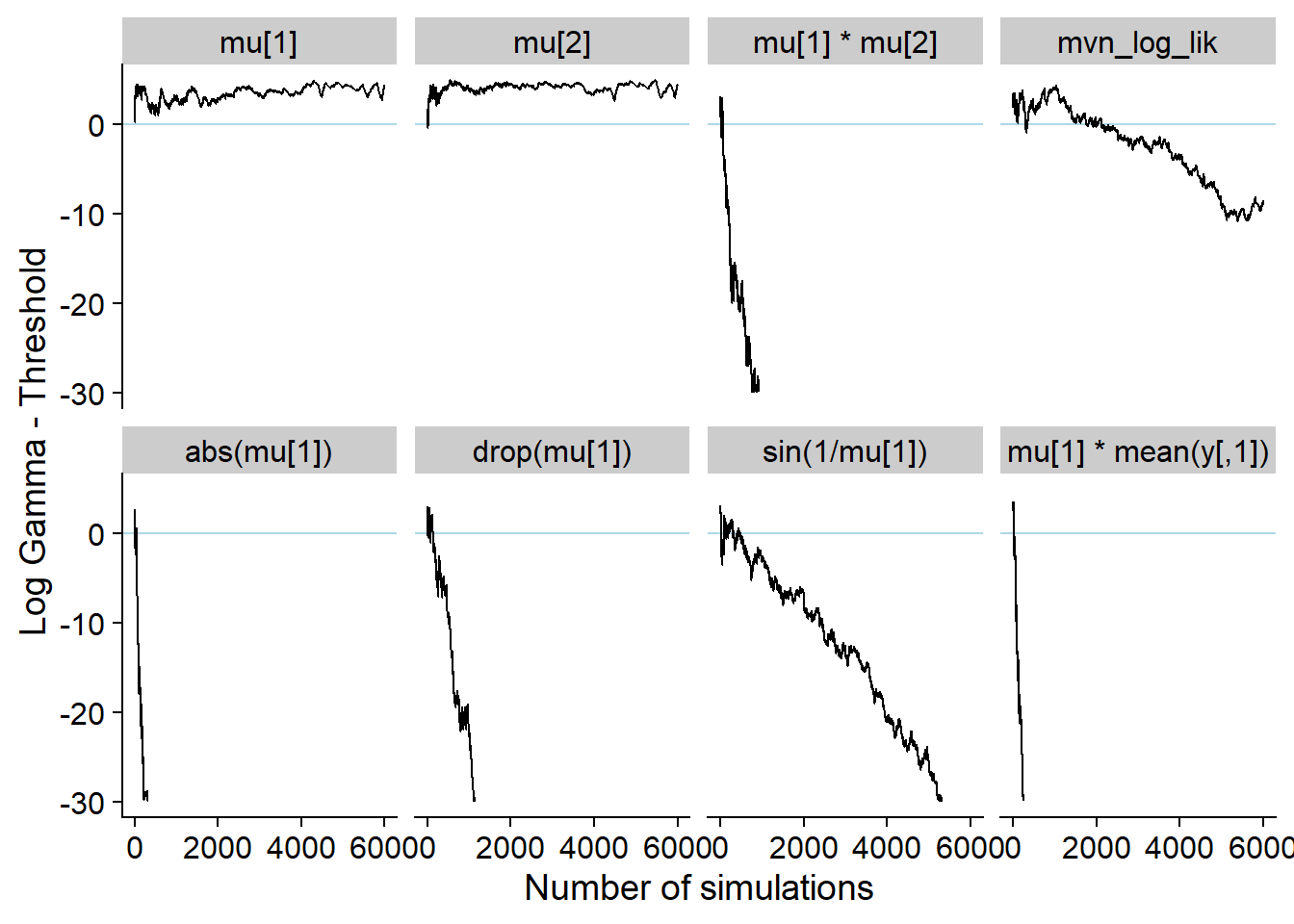

ggsave(file.path(fig_dir, "hist_non_mon_ext.pdf"), p_hist_non_mon_ext, width = hist_plot_width, height = hist_plot_height)

## Warning: Removed 5752 row(s) containing missing values (geom_path).

Small changes compound

Here we add small bias to the correct posterior.

K_changes <- 2
set.seed(5665525)
mvn_sigma_changes <- matrix(0.8, nrow = K_changes, ncol = K_changes)
diag(mvn_sigma_changes) <- 1

ds_changes <- generate_datasets(SBC_generator_function(generator_func_correlated, N = 3, sigma = mvn_sigma_changes), n_sims = 1000)

sampling_func_small_change <- function(y, N_samples, prior_sigma) {
  res_correct <- sampling_func_correct(y, N_samples, prior_sigma)
  K = nrow(prior_sigma)
  bias <- rnorm(K, mean = 0, sd = 0.3)
  res <- res_correct
  for(k in 1:K) {
    res[,k] <- res[,k] + bias[k]  
  }
  res
}

backend_small_change <- my_backend_mvn(sampling_func_small_change, func_extra_args = list(prior_sigma = mvn_sigma_changes))

quants_change <- derived_quantities(sum = sum(mu),
                                      sum_abs = sum(abs(mu)),
                                mvn_log_lik = sum(mvtnorm::dmvnorm(y, mean = mu, sigma = mvn_sigma_changes, log = TRUE)))

res_small_change <- compute_SBC(ds_changes, backend_small_change, dquants = quants, 
                              globals = c(my_backend_mvn_globals, "sampling_func_correct", "mvn_sigma_changes"),
                              cache_mode = "results",
                              cache_location = file.path(cache_dir, paste0("mvn_small_change_", K_changes)))

## Cache file exists but the backend hash differs. Will recompute.

res_small_change <- order_quants(res_small_change)

The diagnostic plots.

plot_rank_hist(res_small_change)

plot_ecdf_diff(res_small_change)

And the history of the gamma statistic:

p_hist_small_change <- plot_log_gamma_history(res_small_change, max_sim_id = 500)
p_hist_small_change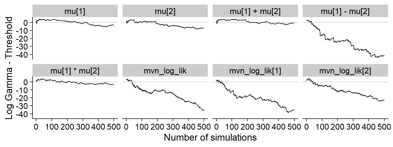

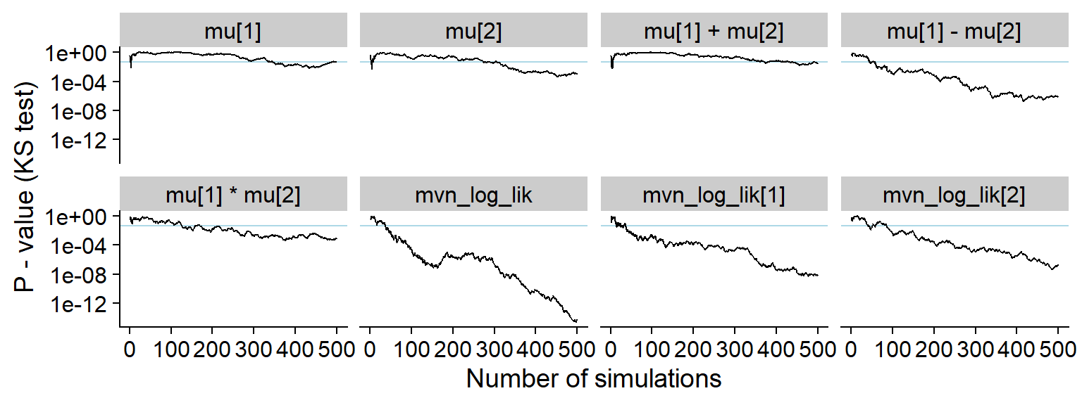
ggsave(file.path(fig_dir, "hist_small_change.pdf"), p_hist_small_change, width = hist_plot_width, height = hist_plot_height)

And the KS p-value - note the reduced sensitivity for e.g. mu[1], mu[2] and mu[1] + mu[2].

plot_ks_test_history(res_small_change, min_sim_id = 0, max_sim_id = 500)